2 - Oscillations
Contents
2 - Oscillations#
Oscillations are ubiquitous in nature. We see it in the motion of springs and pendulums, clearly. But orbital motion of the planets and stellar objects are large scale (both time and space) oscillations. While not obvious, weather patterns, the stock market, and other nonlinear and complex systems exhibit oscillations. Particle oscillations in quantum mechanics are some of the most interesting new physics we have discovered. Check out this short video on the oscillation of neutrinos.
from IPython.display import YouTubeVideo
YouTubeVideo("7fgKBJDMO54", 800, 600)
Neutrino Oscillations#
These neutrino oscillations are incredibly important to the future of high energy and particle physics. Because of their observed oscillation, it is clear the neutrino is not a massless particle, but how much mass is an open question. The work that lead to this discovery was lead by Takaaki Kajita and Arthur McDonald who jointly were awarded the 2015 Nobel Prize in physics.
Current Research at Michigan State
The Physics and Astronomy Department at MSU has a research effort devoted to neutrinos and neutrino oscillations. Some of this work is lead by Prof. Kendall Mahn who works on the Deep Underground Neutrino Experiment (DUNE). The work of her and her team have the potential to break standard model physics and move us into the realm of new particle physics.
The Simple Harmonic Oscillator#
One of the central models of physics is the simple harmonic oscillator; both beloved and ridiculed, it’s hard to deny how often it gets used. At issue is that nature tends towards some equilibrium. Most systems left alone will relax to some equilibrium. Typically, the process minimizes some quantity (e.g., energy) and thus we seek energy wells. These wells may have a complex form, but only depend on position. In 1d, the potential energy (also called the “configuration energy”) is:
A potential energy extrema will have a vanishing first derivative (\(dU/dx=0\)). An energy minimum will have a positive concavity (\(d^2U/dx^2>0\)).
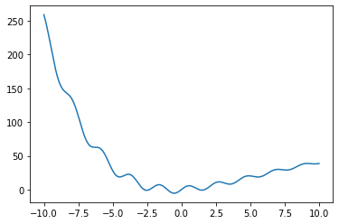
Consider a strange potential energy function:
It is plotted below. Notice the many local potential energy minima. Motion around each of those points can be modeled as a harmonic oscillator.
import numpy as np
import matplotlib.pyplot as plt

x = np.arange(-10,10,0.01)
U = (5*np.sin(3*x)+(x+0.5)**2)*np.exp(-1/10*x)

plt.plot(x,U)
[<matplotlib.lines.Line2D at 0x1199ac730>]
How are we sure we can model each local minimum as an SHO?#
Remember that we are modeling energy minima, so that \(dU/dx=0\) at the point we care about (the local energy minimum). So if we expand the potential in a Taylor series around any minimum energy point (\(x_{localMinEnergy}\)), we find the first non-constant contribution is quadratic,
But, by definition, at a potential energy minimum
We neglect higher order terms, which arguably limits the extent we can predict. That is the space around the potential energy minimum that we can predict with good accuracy depends very much on how much the energy changes near the minimum and how well it can be approximated by a parabola. But, we are left with:
which is an SHO potential energy function.
The SHO mathematical model#
From this potential energy, we find that a reasonable force model (\(F = -dU/dx\)) for a 1D spring system is given by:
where \(k\) is the spring constant for the spring and \(x_0\) is the equilibrium location. As we know from Newton’s second law, if we can argue that this force is the only force or the dominant behavior we are trying to model in a mechanical situation, we have the following ordinary differential equation:
Without much loss, we can recast the problem in terms of the distance from equilibrium
As you will learn this is not a problem for vertically hanging springs near the surface of the Earth because the gravitational force is constant and depends on the mass of the hanging weight.
The SHO mathematical model
Finding the general solution#
We can solve this using our typical approach to 2nd order linear ODEs; guess the form of the solution and check it. You might have done this in the past with functions of \(\sin\) and \(\cos\). Here, we will introduce the complex form of the solution as a compliment.
Assume: \(s(t) = A\exp(i\omega t)\) As we will learn this form is a good guess for linear ODEs. You might be worried about the \(i\), which is a complex number \(i = \sqrt{-1}\). That’s ok, for now, let’s use it. Then we will see how it connects.
Putting in the guessed solution (“the ansatz”) gives:
So that,
This solution is consistent with the model (i.e., solves the differential equation) if we set \(\omega\) and notice it is exclusively positive:
Thus, \(s(t) = A\exp(i\sqrt{\frac{k}{m}} t)\) is a solution to this problem. Notice we have to set \(A\) using initial conditions for the problem. This is called a initial value problem in mathematics.
What about that pesky imaginary part?#
Our complex formulation is consistent with the \(\sin\) and \(\cos\) approach you have used in the past. You might have heard about the Euler formulation; it is one of the most important relationships in mathematics [Nahin, 2011, Stipp, 2017]. We will get into it more later. It appears below:
Leonhard Euler’s famous formula
Thus, we know that our solution gives rise to real sinusoidal solutions of the form:
This probably doesn’t look quite right…there’s an \(i\) in the solution for real physical motion! We will get to that, but we need the initial conditions to do so. More importantly, there’s only one free parameter in our current solution, \(A\). Given that this equation is a solution, is it the only solution?
The order of your differential equation matters#
You probably already know that our general solution for the SHO is:
Or written in a way that is more often presented:
where we have made clear that the free parameters \(A\) and \(B\) are not equal to \(A'\) and \(B'\), respectively. Regardless, notice there’s two free parameters in these formula. That is because we are solving a two dimensional linear ODE. Because there’s two derivatives on \(s\) (i.e., \(\ddot{s}\)), we expect to have two free parameters that are set by the intial conditions. This is characteristic of an initial value problem.
Important Tip
The number of free parameters that are set by problem conditions in an initial value problem is determined by the order of the differential equation.
Second order? Two conditions needed. Two free parameters to determine. Fourth order? Four conditions needed. Four free parameters to determine.
More Resources#
If you are feeling less comfortable with the harmonic oscillator or it’s been some time, I think Prof. Ten-Jie Lee’s lecture is very good. It’s long (a full 50 minutes), but here’s some key points:
About 10 minutes in, he derives the full solution (we will not do this)
About 17 minutes in, he shows how to get particular solutions with initial conditions (we will do this)
About 26 minutes in, he completes an example where he shows how to Taylor approximate a potential to use the SHO model (we will do something like this)
About 40 minutes in, he discusses the different forms of the solutions (we will do this)
About 43 minutes in, he brings in complex analysis (we will do this)
YouTubeVideo("4ysFC9vd3GE", 800, 600)