06 Sept 22 - Activity: Investigating the Simple Harmonic Oscillator#

Reminders of the SHO and Introduction to Dynamical Systems#

Look for ✅ Do this

The SHO mathematical model#

We have seen for the canonical one-dimensional harmonic oscillator is described by the following 2nd order linear differential equation:

\[m\ddot{s} = -k{s}\]

where \(s\) represents the distance from the oscillators equilibrium position. It’s important to note that this model for a linear restoring force gives rise to at econd order differential equation. As you will see, there would be no ability for cycles or recurrent behavior without two dimensions (the two dimensions here are the position, \(s\), and velocity of the oscillator, \(\dot{s}\)). It is also important that the differential equation is linear.

Linearity of differential equations#

This is something that is easy to confuse because we use the term linear in different ways at different times. In many cases this prompts us to think of a line, so that we might think the only linear differential equations are ones where the variable of interest (in this case the position of the oscillator) appears only linearly in the equation.

Warning

So you might think that Nth order differential equations of the form:

\[\dfrac{d^n x}{dt^n} = c\;x\]

are the only ones that are linear. Note for the harmonic oscillator \(n=2\).

That is not the case and this is key.

The linearity refers to the fact that we can write the differential equation as a linear combination of the derivatives.

Tip

So an \(N\)th linear differential equation (e.g., for position and time) can have the general form:

\[\sum_{i=0}^N a_i(t)\dfrac{d^ix}{dt} = f(t)\]

where \(\dfrac{d^ix}{dt}\) is the \(i\)th derivative of \(x\) (e.g., \(i=0\), \(\dfrac{d^0x}{dt}=x\); \(i=1\), \(\dfrac{d^0x}{dt}=\dfrac{dx}{dt}\)) The coefficients are allowed to depend explicitly on time (i.e., \(a_i(t)\); you have probably seen constant coefficients in the past (where \(\dfrac{da_i(t)}{dt}=0\), i.e., \(a_i(t) =\) constant). In addition, as you can explore later, the system can be driven by a function that depends only on time (e.g., some forcing function, \(f(t)\)).

Why does linearity matter?#

Because much of nature can be modeled with linear differential equations (or approximately so) and linear differential equations have really nice solution properties. *The solutions to linear differential equations are holonomic functions. This is just a fancy word for functions you know like polynomials, sine, cosine, exponentiale, and some special functions (e.g., Airy, Bessel, hypergeometric). But these solutions are really important because they are smooth as are their derivatives, so they have really nice properties.

In many cases, we can lean on strong properties dervied from linearity:

Uniqueness: If we find a solution to the differential equation and it satisfies the boundary/initial conditions, we are guaranteed that this is the only solution.
Linear combinations: The linear nature of the differential equation means linear combinations of general solutions are unchanged. We can build solutions from known general solutions.

The Cauchy-Kowaleski theorem

This theorem is typically called the Cauchy theorem (or the uniqueness theorem) for Augustin Louis-Cachy, a French mathematician who contributed much to the field of complex analysis. However, Cauchy only proved this theorem in a special case. A Russian Mathematician, Sofya Kovalevskaya, who was the first woman to earn a PhD in Mathematics (earned 1874, University of Göttingen), proved the theorem, in general, in her dissertation.

So, it is really the “Kovalevskaya-Cauchy” theorem.

General Solution to the SHO#

We can start with the differential equation:

\[\ddot{x} = -\omega^2 x\]

where \(x\) is the position relative to equilibrium and \(\omega^2 = k/m\). We know this is a linear, second-order ODE, so we expect the solutions to be holonomic functions - that is, many of the functions we have seen before. Moreover, we need something that when we take two derivatives, we get the same functions back.

This is a key to suggest \(\sin\) and \(\cos\) as our proposed linear combination.

Now, we have to decide how to do that. Because ANY linear combination is a good starting guess, but not all of them a reasonable guesses. How do we decide?

Discussion Question#

✅ Do this

Below are several choices of potential general solution guesses, called “ansatz” in many books and classes. Which of them will work for us? How do you know? Discuss with your neighbors Demonstrate that one solution you chose works.

\[x(t) = A\cos(\omega t)\]

\[x(t) = B\sin(\omega t)\]

\[x(t) = A\cos(\omega t)+B\sin(\omega t)\]

\[x(t) = B\sin(\omega t+ \phi_B)\]

\[x(t) = \sum_i^N A_i\cos(\omega_i t) + B_i\sin(\omega_i t)\]

What other general solution forms will work?

Particular Solutions#

Let’s pick two general solutions:

\[x(t) = A\cos(\omega t) + B\sin(\omega t)\]

\[x(t) = C\sin(\omega t + \phi_C)\]

✅ Do this

For an SHO that is pulled to a point \(x_0\) and let go at \(t=0\), find the particular solutions using both general forms. Compare and contrast these solutions with your neighbor. What do you notice about them? How can they be made compatible with each other?
Make a plot (in this notebook) of both solutions for an SHO with frequency of 100Hz that starts at \(x_0 =\) 0.1m
Adjust the starting location and frequency, what do you notice?
If you have time, create another solution for an SHO that is put into motion with a velocity of +0.1m/s at \(x_0=0\) at \(t=0\).

import numpy as np
import matplotlib.pyplot as plt

#################################
# Adjust code to fit your needs #
#################################

t = np.arange(0,10,0.1)
x = t**2

plt.plot(t,x)

[<matplotlib.lines.Line2D at 0x116fd8ee0>]

../../_images/activity-SHO_and_dynamical_systems_7_1.png

SHO properties#

You have likely work with the SHO in other contexts. You have learned about a variety of aspects of the SHO. Talk with your neighbor about different things you all know about the properties of the SHO (it’s motion, it’s energy, etc.).

✅ Do this

Decide on one or two things to investigate and plot with respect to the SHO. Be ready to explain your figure, to discuss how to improve it, and what we can claim from it.

import numpy as np
import matplotlib.pyplot as plt

#################################
# Adjust code to fit your needs #
#################################

t = np.arange(0,10,0.1)
x = t**2

plt.plot(t,x)

[<matplotlib.lines.Line2D at 0x1171753c0>]

../../_images/activity-SHO_and_dynamical_systems_10_1.png

Shifting gears#

We will come back to the SHO and how we complicate it soon, but we are going to use our knowledge of the SHO to bring in a new analytical tool: Dynamical Systems.

Introduction to Dynamical Systems#

Dynamical systems is a branch of mathematics that seeks to investigate the time dependence of a system and characterize the families of trajectories the system can have. We don’t often solve the system for a given set of conditions in dynamical systems work. Instead, we want to uncover the families of possible solutions for a system to see what kinds of things it can do. An excellent book on this subject that we will draw from is Strogatz’s book on Nonlinear Dynamics [Strogatz, 2018]; i highly recommend you find a copy for yourself.

Geometric Thinking and Phase Portraits#

One of the first things we will use to investigate the SHO from a dynamical systems perspective is the phase portrait, where we will plot the velocity against the position. We can use the phase portrait to tell us what families of solutions we might expect to see.

Phase portraits are quite useful for second order differential equations (or any two-dimensional system) because we frequenty use and interpret 2D graphs. Notice that we focused on “2nd order differential equations” not “linear 2nd order.” That is because, as we will see, phase portraits are particularly useful for nonlinear 2nd order differential equations.

Example#

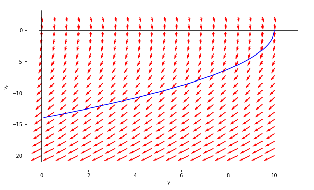
Consider a falling object in one-dimension. A model for free fall where we define \(+y\) in the upward direction (away from the ground) and we neglect influences beyond the gravitational interaction leads us to:

\[\ddot{y} = -g\]

where \(g \equiv +9.8\) m/s (that is, \(g>0\) with these definitions).

We can make a phase portrait by considering how the position, \(y\), and velocity, \(v_y\), change. We represent those changes with arrows in the same space. To do this we must separate our 2nd order ODE into two 1st order ODEs (one for \(y\) and one for \(v_y\)). That is relatively straightforward for this case:

\[\dot{y} = v_y\]

\[\dot{v_y} = -g\]

Plot the vector field#

The phase portrait can be represented by arrows that indicate how the system moves through phase space. Below we have written the code to make the phase portrait for this system.

def GravPhasePortrait(Y,t):

## GravPhase Portrait takes the position variable y1 and velocity variable y2 
## and returns the vectors that describe how each change in the phase space
    
    y1, y2 = Y
    vectors = [y2, -9.8] ## Specific to the problem
    return vectors

y1 = np.linspace(0.0, 10.0, 20)
y2 = np.linspace(-20.0, 2.0, 20)

## A meshgrid makes pairs of points in a 2D space that 
## we can use to compute the value of a vector at a 
## location in 2D space

Y1, Y2 = np.meshgrid(y1, y2)

t = 0

u, v = np.zeros(Y1.shape), np.zeros(Y2.shape)

X, Y = Y1.shape

## We need to compute the vectors in the space
## This loop steps through each grid point (not two loops)
## to do this calculation

for i in range(X):
    for j in range(Y):
        x = Y1[i, j]
        y = Y2[i, j]
        vectors = GravPhasePortrait([x, y], t)
        u[i,j] = vectors[0]
        v[i,j] = vectors[1]

## A quiver plot is a common way to present a vector field
## THe arrows indicate the direction of the "flow" of the dynamical system  
ax = plt.figure(figsize=(10,6))
Q = plt.quiver(Y1, Y2, u, v, color='r')

plt.plot([-.1,11],[0,0],'-k')
plt.plot([0,0],[-21,3],'-k')
plt.xlabel('$y$')
plt.ylabel('$v_y$')

## Plotting a trajectory
y0, v0, g = 10, 0, 9.8

## To do this we solved the kinematic equations for
## the velocity in terms of the position
## In some cases, we can do this, in others,
## we will have generate data based on time 
## and plot things together (see below), but a more
## useful tool is to numerically solve the problem

y_traj = np.linspace(0.1,10,100)
v_traj = -1*np.sqrt(v0**2-2*g*(y_traj-y0)) 
#print(2*g*(y_traj-y0)**2)
plt.plot(y_traj,v_traj,'-b')

[<matplotlib.lines.Line2D at 0x1171cb9d0>]

../../_images/activity-SHO_and_dynamical_systems_13_1.png

Discussion Question#

✅ Do this

Work with your neighbors to make sense of this code and the resulting plot. Try to write down what each line is doing and explain it to each other. Then, try to interpret the plot. Adjust the parameters and see what happens? What can you learn about a falling object from this?

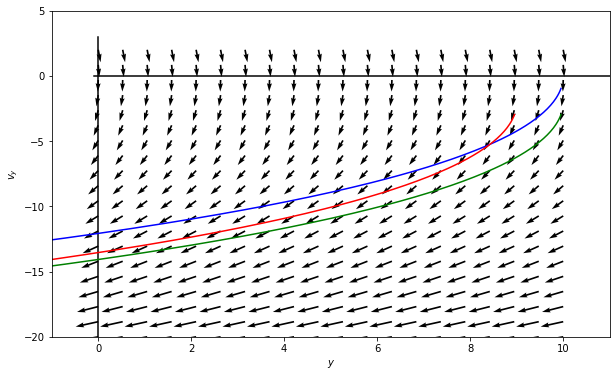
Adding Drag#

We are going to explore ODEs that have multiple terms next week. But ti get started consider a 1 dimensional fall object that experiences linear drag. The mathematical model we use for this is given by the following linear 2nd order differential equation.

\[m\ddot{x} = -m*g + \beta*\dot{x}\]

Linear drag is the simplest model of drag. It is useful in only a few cases (small and slow moving objects). The REynolds number characterizes the relationship between inertial (weight) and viscous (drag) forces. Low Reynolds? Laminar flow! High Reynolds? Turbulence! One of the most interesting papers about this is called “Life at Low Reynolds Number” by E.M. Purcell. It’s a great, short read.

We will show (not today) that we can derive trajectories for this solution of the form:

\[v(t) = -\dfrac{g}{\beta}+\dfrac{g}{\beta} e^{-\beta t}\]

\[y(t) = \int v(t) dt = y_0 - \dfrac{g}{\beta}t + \dfrac{g}{\beta^2}\left(1-e^{-\beta t}\right)\]

Below we have constructed a code that explores the phase portrait of a falling object with drag

Discussion Question#

✅ Do this

Work with your neighbors to make sense of this code and the resulting plots. Try to write down what each line is doing (you’ve done this already) and explain it to each other. Then, try to interpret the plots. Adjust the parameters and see what happens? What can you learn about a falling object with drag from this?

def GravWithLinearDragPhasePortrait(Y,t,beta = 0.1):

## GravWithLinearDragPhasePortrait takes the position variable y1 and velocity variable y2 
## and returns the vectors that describe how each change in the phase space
## the parameter beta lets you adjust the strength of the linear drag
    
    y1, y2 = Y
    vectors = [y2, -9.8-beta*y2] ## Specific to the problem
    return vectors

beta = 0.3 ## DRAG COEFF

###########################
# All the same code below #
###########################

y1 = np.linspace(0.0, 10.0, 20)
y2 = np.linspace(-20.0, 2.0, 20)

Y1, Y2 = np.meshgrid(y1, y2)

t = 0

u, v = np.zeros(Y1.shape), np.zeros(Y2.shape)

X, Y = Y1.shape

for i in range(X):
    for j in range(Y):
        x = Y1[i, j]
        y = Y2[i, j]
        vectors = GravWithLinearDragPhasePortrait([x, y], t, beta)
        u[i,j] = vectors[0]
        v[i,j] = vectors[1]

ax = plt.figure(figsize=(10,6))
Q = plt.quiver(Y1, Y2, u, v, color='k')

plt.plot([-.1,11],[0,0],'-k')
plt.plot([0,0],[-21,3],'-k')
plt.xlabel('$y$')
plt.ylabel('$v_y$')

### Trajectory
t = np.linspace(0.1,10,1000)

y0, v0, g = 10.0, 0.0, 9.8
v_traj = v0-g/beta+(g/beta)*np.exp(-beta*t)
y_traj = y0 - (g/beta)*t + (g/beta**2)*(1-np.exp(-beta*t))

y0, v0, g = 10.0, -2.0, 9.8
v_traj2 = v0-g/beta+(g/beta)*np.exp(-beta*t)
y_traj2 = y0 - (g/beta)*t + (g/beta**2)*(1-np.exp(-beta*t))

y0, v0, g = 9.0, -2.0, 9.8
v_traj3 = v0-g/beta+(g/beta)*np.exp(-beta*t)
y_traj3 = y0 - (g/beta)*t + (g/beta**2)*(1-np.exp(-beta*t))


plt.plot(y_traj, v_traj,'-b')
plt.plot(y_traj2, v_traj2,'-g')
plt.plot(y_traj3, v_traj3,'-r')


plt.xlabel('$y$')
plt.ylabel('$v_y$')

plt.xlim([-1, 11])
plt.ylim([-20, 5])

(-20.0, 5.0)

../../_images/activity-SHO_and_dynamical_systems_16_1.png

Discussion Question#

✅ Do this

Compare the phase potraits of the no drag and drag case. What do they tell you about the families of solutions? Discuss with your neighbors.

Back to the SHO#

✅ Do this

Use the above code to make a phase portrait of the SHO. Add trajectories to the portrait. What does this tell you about the SHO?

## Your code here

Lingering Questions#

✅ Do this

What lingering questions do you have? What should we explore more?

Notes here

Mathematical Modeling in Physics

06 Sept 22 - Activity: Investigating the Simple Harmonic Oscillator

Contents

06 Sept 22 - Activity: Investigating the Simple Harmonic Oscillator#

Reminders of the SHO and Introduction to Dynamical Systems#

The SHO mathematical model#

Linearity of differential equations#

Why does linearity matter?#

General Solution to the SHO#

Discussion Question#

Particular Solutions#

SHO properties#

Shifting gears#

Introduction to Dynamical Systems#

Geometric Thinking and Phase Portraits#

Example#

Plot the vector field#

Discussion Question#

Adding Drag#

Discussion Question#

Discussion Question#

Back to the SHO#

Lingering Questions#