11 Oct 22 - Activity: Normal Modes of 3 Coupled Oscillators
Contents
11 Oct 22 - Activity: Normal Modes of 3 Coupled Oscillators#
Now that we have discussed and built some facility with Lagrangian dynamics, let’s see how using it makes our study of normal modes much simpler than Newtonian mechanics. We will couple this analysis to solving an eigenvalue problem by guessing the form of the solutions. This technique is very common in theoretical physics with different guesses for the solution forms giving rise to different eigenvalue problems (e.g., Bessel functions for 2D surface problems or Hermite polynomials for the Quantum Harmonic Oscillator.
Three Coupled Oscillators#
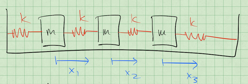
Consider the setup below consisting of three masses connected by springs to each other. We intend to find the normal modes of the system by denoting each mass’s displacement (\(x_1\), \(x_2\), and \(x_3\)).
Finding the Normal Mode Frequencies#
✅ Do this
This is not magic as we will see, it follows from our choices of solution. Here’s the steps and what you might notice about them:
Guess what the normal modes might look like? Write your guesses down; how should the masses move? (It’s ok if you are not sure about all of them, try to determine one of them)
Write down the energy for the whole system, \(T\) and \(U\) (We have done this before, but not for this many particles)
Use the Euler-Lagrange Equation to find the equations of motion for \(x_1\), \(x_2\), and \(x_3\). (We have done this lots, so make sure it feels solid)
Reformulate the equations of motion as a matrix equation \(\ddot{\mathbf{x}} = \mathbf{A} \mathbf{x}\). What is \(\mathbf{A}\)? (We have done this, but only quickly, so take your time)
Consider solutions of the form \(Ce^{i{\omega}t}\), plug that into \(x_1\), \(x_2\), and \(x_3\) to show you get \(\mathbf{A}\mathbf{x} = -\omega^2 \mathbf{x}\). (We have not done this, we just assumed it works! It’s ok if this is annoying, we only have to show it once.)
Find the normal mode frequencies by taking the determinant of \(\mathbf{A} - \mathbf{I}\lambda\). Note that this produces the following definition: \(\lambda = -\omega^2\) (We have not done this together and we can if it’s confusing.)
Finding the Normal Modes Amplitudes#
Ok, now we need to find the normal mode amplitudes. That is we assumed sinusoidal oscillations, but at what amplitudes? We will show how to do this with one frequency (\(\omega_1\)), and then break up the work of the the other two. These frequencies are:
✅ Do this
After we do the first one, pick another frequencies and repeat. Answer the follow questions:
What does this motion physically look like? What are the masses doing?
How does the frequency of oscillation make sense? Why is it higher or lower than \(\omega_A\)?