13 Oct 22 - Activity: Normal Modes of N Coupled Oscillators

Now that we have developed solutions for the 3 coupled oscillators, let’s try to reproduce that work numerically and plots the modes to make sense of what they are doing for us.

We can then apply these tools to \(N\) identically coupled 1D oscillators.

Three Coupled Oscillators

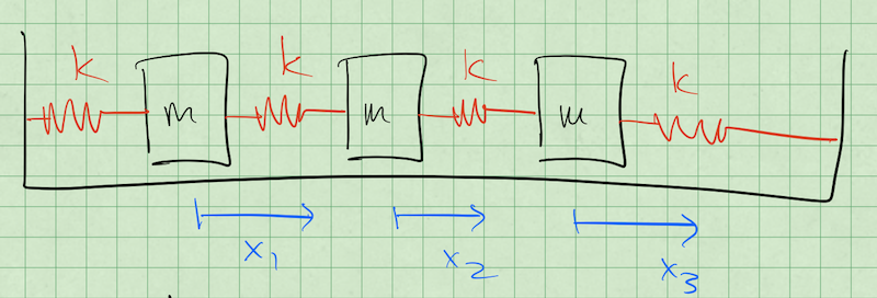
Consider the setup below consisting of three masses connected by springs to each other. We intend to find the normal modes of the system by denoting each mass’s displacement (\(x_1\), \(x_2\), and \(x_3\)).

We start by importing the libraries that we need.

import numpy as np
import matplotlib.pyplot as plt
import numpy.linalg as la ## For the numerical eigenvalue methods
from sympy import * ## For symbolic eigenvalue methods
init_printing(use_unicode=True)  ## display nice math

Finding the Eigenvalues and Eigenvectors

We reduced our normal mode problem to the following:

\[\mathbf{A}\mathbf{x} = -\omega^2\mathbf{x}\]

And earlier we found these eigenvalues and eigenvectors for the 3 Oscillator model:

\[\omega_A = 2\dfrac{k}{m}; \qquad \omega_B = \left(2-\sqrt{2}\right)\dfrac{k}{m}; \qquad \omega_C = \left(2+\sqrt{2}\right)\dfrac{k}{m}\qquad\]

Python has two main libraries for helping us find these numerically. One is numpy.linalg, which is a powerful set of linear algebra tools that are used widely. The other is sympy, which is a symbolic calculator like Mathematica. Both will help you find eigenvalues and eigenvectors, but do so in entirely different ways.

• numpy.linalg will use the common numerical tools that decompose matrices. For example, LU decomposition is one of the most common techniques to use for symmetric and Hermitian matrices, which are the most common in physics.

• sympy is a symbolic calculator, that attempts to determine a closed form solution for the eigenvalues. These methods are often proprietary (e.g., Mathematica and Matlab), but the source code for sympy is available to review.

At issue is that each of these methods requires a slight different input. The first method will take a numpy matrix, but the second requires a sympy matrix, which can we easily constructed from our numpy matrix.

Below, we form both matrices.

M = np.matrix([[-2, 1, 0], [1, -2, 1], [0, 1, -2]]) ## numpy matrix
M2 = Matrix(M) ## Take numpy matrix and make it a sympy one
print(M)
print(M2)

[[-2  1  0]
 [ 1 -2  1]
 [ 0  1 -2]]
Matrix([[-2, 1, 0], [1, -2, 1], [0, 1, -2]])

Finding eigenvalues with numpy.lingalg is quite simple. We just call eigenvals, eigenvecs = la.eig(M). Note they are numericaly values. Also, these eigenvectors are normalized. Do you notice anything strange?

eigenvals, eigenvecs = la.eig(M)
print(eigenvals)
print(eigenvecs)

[-3.41421356 -2.         -0.58578644]
[[ 5.00000000e-01  7.07106781e-01  5.00000000e-01]
 [-7.07106781e-01 -4.05925293e-16  7.07106781e-01]
 [ 5.00000000e-01 -7.07106781e-01  5.00000000e-01]]

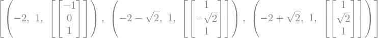
Finding the eigenvectors and eigenvalues with sympy is just as simple. Notice that these are symbolic and the eigenvectors are NOT normalized.

M2.eigenvects()

Plotting the modes

Awesome. Now we have our modes, but what do they mean? Remember, in a given mode every object oscillates at the mode frequency, just with different amplitudes. That means everyone has the following form:

\[A\cos(\omega t)\]

just with different \(A\)’s. So plot the motion of each mass in each mode. Make sure you have the right frequencies with the right modes.

## Analysis and Plotting code here

Extending your work

Given what we have done thus far, you can see that we could easily construct the matrix for a \(N\) dimensional chain of 1D oscillators. So let’s do that.

Repeat this analysis for a set of \(N\) oscillators. Your code should be able to:

1. Take a value of \(N\) and construct the right matrix representation

2. Find the eigenvalues and eigenvectors for this matrix.

3. (BONUS) plots the modes automatically

4. (CHALLENGE) time the execution of the analysis

Be careful not to pick to large of an \(N\) value to work with because you could melt your CPU easily. Make sure your code can do something like \(N=10\). If you get the timing working, plot time vs number of objects to see how the problem scales with more oscillators.

## Your code here

Even further

These models can be used with lattices (solid objects). Draw a sketch of 4 oscillators in a plane connected together in a square shape. Write down the energy equations for this system (assume the springs do not move laterally much). What do the EOMs look like?