3 Oct 23 - Notes: Electric Potential - a scalar field#
We’ve seen that there’s a lot of challenges with solving field problems where the fields are vectors and described by partial differential equations. The electric and magnetic field are vector fields that have a size and direction are every points in space. They are described by a set of 4 partial differential equations, Maxwell’s Equations. In Cartesian coordinates, these equations are described by 8 coupled partial differential equations.
Electrostatics#
In electrostatic situations, where charges don’t move, we’ve seen that the equations that describe the electric field are simplified to:
In general, in Cartesian coordinates, these are still four partial differential equations. However, the electric field is curl-less, so we can write it as the gradient of a scalar field, \(V\):
We might prefer to work with this scalar field, \(V\), rather than the vector field, \(\vec{E}\), because it is a simpler object to work with. There’s a number of tools we can use to find the potential and then we take the gradient to find the electric field.
Electric Potential#
Parth G has a really nice video on the conceptual elements of electric potential, we will concern ourselves with more mathematical aspects as we move forward.
Non-Commercial Link: https://inv.tux.pizza/watch?v=7rjAtuwxrEA
Commercial Link: https://youtube.com/watch?v=7rjAtuwxrEA
The electric potential is the scalar field that we have developed. One thing to note about it, is that it is only defined up to a constant. That is because when we take the gradient, and constant will drop out. This is really important when stitching together solutions from multiple sources. They need to all have the same “zero of potential.”
With the definition, \(\vec{E}(x,y,z) = -\nabla V(x,y,z)\), we can conclude the following:
where \(\nabla^2\) is the Laplacian operator. This is Poisson’s Equation, a well-studied second order partial differential equation. When used in electrostatics, it is a central equation for solving for the electric potential. In addition, we can integrate to show that:
where the line integral is taken along a path from one point to another. For the electric field, this is independent of path, so we can write:
And
which is a direct results of applying Stokes’ Theorem to the curl-less electric field, and indicates that the electric field is conservative.
Getting to Laplace’s Equation#
Poisson’s Equation is a description of a scalar potential (e.g., the electric potential) and how it relates to sources of the potential (e.g., charges). This is a local description of the field. At every point, the Laplacian can be computed (for well-behaved functions) and it indicates a source or lack of sources. For example, in empty space with no charges, the Laplacian is zero everywhere.
So if we imagine setting up charges far from the place we are interested in finding the electric potential, we have an equation that is describes that space.
This is Laplace’s equation and is a commonly occurring equation in physics. In fact, as we saw here, it shows up anytime we find local situations where the charges are absent. So the idea is that charges are far away setting the potential at the boundaries (hence, calling these boundary value problems). The idea is that the PDE is solved in the region of interest often giving some general solution in the form of an infinite sum. The boundary conditions are then used to determine the coefficients in the solution, giving a unique solution. Because Laplace’s equation is a linear PDE, the superposition principle applies, so we can add solutions together to get new solutions.
A typical problem#
It might seem odd to have an equation that is everywhere equal to zero and somehow suggest it produces non-zero solutions. But remember that it is a PDE that describes the second derivatives of this scalar function,
It turns out there’s lots of functions that will satisfy that differential equation. And it’s mostly a matter of if the function fits the boundary conditions. Let’s look at a typical problem.
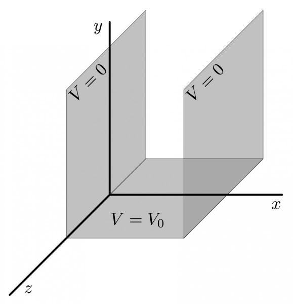 Image from University of Guelph
Here is a “gutter” where the electric potential for different sides of the gutter are set. Laplace’s equation applies inside the gutter. So the idea is to find a solution that satisfies Laplace’s equation and the boundary conditions. We will develop this solution in class, but the representative results look like this:
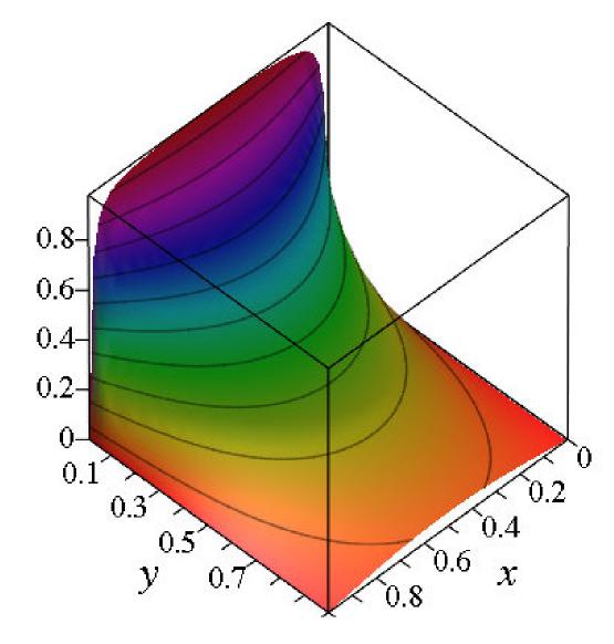 Image from University of Guelph
Separation of Variables#
One of the key analytical tools that we have for Laplace’s Equation is the separation of variables method of solving PDEs. We posit an ansatz in which the solution is a product of functions of the individual variables. For example, in Cartesian coordinates, we might write:
And then we plug that into Laplace’s equation and see if we can find solutions. In this case, we get:
which we divide by \(XYZ\) to obtain the following expression:
Here each partial derivative is a of a pure function of a single variable. So we can conclude that each term is a constant that sum to zero. We can write this as:
where \(k_x^2 + k_y^2 + k_z^2 = 0\). We have converted our problem to a set of 3 ODEs that we know how to solve. We can then solve each of these equations separately and show a general solution is:
where \(A,B,C,D,E,F,G\) are constants. We can then use the boundary conditions to determine the constants. Notice we wrote these as complex exponentials, those are sinusoidal or exponential solutions depending on if the resulting \(k\)’s are real or complex. The electric potential is a real measurable quantity.
This general approach is well known and well-traveled territory. It’s working with these boundary conditions that can be tricky, and that we will practice. We will find that for most cases that we end up with infinite sums of these solutions. We will also find that we can use the orthogonality of the solutions to simplify the solutions.
We should not suggest that every PDE can be solved with separation of variables, but rather that:
Separation of variables is a powerful tool for solving PDEs that you can try, but it might not work.
It is a tool that can produce general solutions to Laplace’s Equation when the Laplacian is separable in the given coordinate system.
It cannot be used for some problems (e.g., when the boundary conditions cannot be expressed as Neumann or Dirichlet boundary conditions).
Other Coordinate Systems#
It turns out the trick of positing a solution that is a product of functions of the individual variables works in other coordinate systems as well. For example, in cylindrical coordinates, we might write:
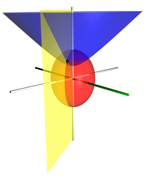
Or in spherical coordinates, we might write:
It turns out both of these are separable in their respective coordinate systems. We will work through some examples of spherical coordinates in class as it forms the basis of the Multipole Expansion, which is a critical mathematical tool with wide applications.
This idea of funding general solutions to Laplace’s equation in known orthogonal coordinate systems remains incredible common. Experimental setups and theoretical models often have situations where Laplace’s equation is relevant and there is a symmetry that can be exploited to find solutions. Laplace’s equation is separable in 13 coordinate systems. You can find some of the more exotic equations and coordinate systems here. Check out the Prolate Spheroidal coordinates, which are used in nuclear physics when the nucleus is deformed.
Additional Resources#
Textbook Chapter#
The University of Guelph provides free notes in physics. Here’s the relevant chapter on Laplace’s Equation. It is also where some of the figures were taken from.
Videos Derivations#
Steve Brunton at Washington has some really great videos on the derivations associated with PDEs like those above.
Possion’s and Laplace’s Equation#
Non-Commercial Link: https://inv.tux.pizza/watch?v=nmvs0vrBT18?
Commercial Link: https://youtube.com/watch?v=nmvs0vrBT18?
Separation of Variables#
Non-Commercial Link: https://inv.tux.pizza/watch?v=VjWtMl6vQ3Q
Commercial Link: https://youtube.com/watch?v=VjWtMl6vQ3Q