7 Nov 23 - Activity: The Fast Fourier Transform

We have shown how to decompose a signal using a Fourier series decomposition:

\[V(t) = \sum_{n=-\infty}^{\infty} c_n e^{i n \omega t}\]

where we find the Fourier coefficients \(c_n\) by integrating over the period of the signal (performing a Fourier transform of the signal):

\[c_n = \frac{1}{T} \int_0^T V(t) e^{-i n \omega t} dt\]

Extracting the Fourier coefficients

We wrote some code earlier to perform the Fourier transform of a signal and obtain the coefficients. We will see how to do that using the scipy library later, but let’s produce these results first without it. We are going to prepare several test signals, but you will need to make more.

Test Signals

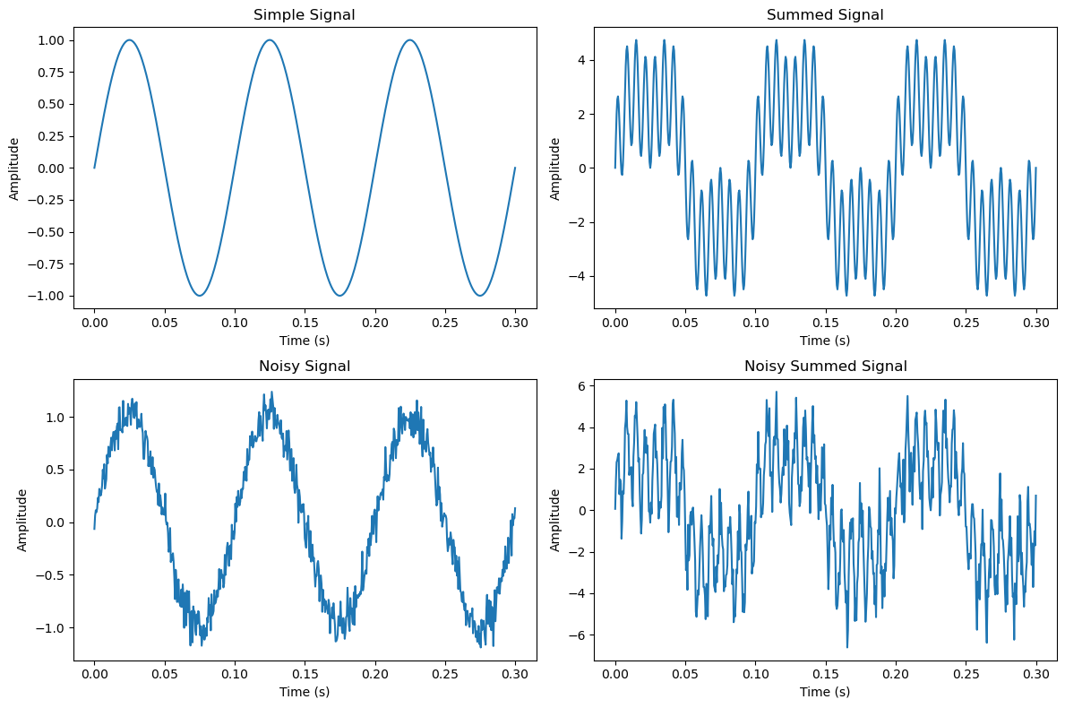
The test signals we are going to use are:

• A sine wave with frequency 10 Hz and amplitude 1 V: \(V(t) = A\sin(2 \pi f t)\)

• A sum of 3 in-phase sine waves with frequencies 10 Hz, 15 Hz, and 30Hz, with amplitudes, 3V, 2V, and 1V respectively: \(V(t) = A_1 \sin(2 \pi f_1 t) + A_2 \sin(2 \pi f_2 t) + A_3 \sin(2 \pi f_3 t)\)

• Both of these signals with random noise added to them.

Below we import the libraries we need and define the functions we will use to generate the signals.

import numpy as np
import matplotlib.pyplot as plt
import random

# Define the functions to create signals
def simple_signal(t, A=1, f=1):
    """Creates a simple sinusoidal signal."""
    return A*np.sin(2 * np.pi * f* t)

def summed_signal(t, A, f):
    """Creates a more complex signal with multiple frequencies."""
    return A[0] * np.sin(2 * np.pi * f[0]*t) + A[1] * np.sin(2 * np.pi * f[1]*t/T0) + A[2]*np.sin(2 * np.pi * f[2]*t)

def noisy_signal(t, A=1, f=1, B=1):
    """Creates a simple signal with random noise."""
    random.seed(42) # seed keeps the random numbers the same each time
    noise = B*np.random.normal(0, 1, len(t)) 
    return simple_signal(t, A, f) + noise

def noisy_summed_signal(t, A, f, B=1):
    """Creates a simple signal with random noise."""
    random.seed(42) # seed keeps the random numbers the same each time
    noise = B*np.random.normal(0, 1, len(t))
    return summed_signal(t, A, f) + noise

Let’s create those signals and plot them.

# Set the sample rate and time
dt = 0.0005  # Sampling frequency
T0 = 0.1 # Signal period
T = 3.0*T0  # Sample time length
t = np.arange(0, T, dt)  # Time points

fsimple = 10
Asimple = 1

f = np.array([10, 15, 30])
A = np.array([3, 2, 1])

simple = simple_signal(t, Asimple, fsimple)
summed = summed_signal(t, A, f)

simple_noise = 0.1
summed_noise = 0.8

noisy = noisy_signal(t, Asimple, fsimple, simple_noise)
noisy_summed = noisy_summed_signal(t, A, f, summed_noise)

plt.figure(figsize=(12, 8))
plt.subplot(2, 2, 1)
plt.plot(t, simple)
plt.title('Simple Signal')
plt.xlabel('Time (s)')
plt.ylabel('Amplitude')

plt.subplot(2, 2, 2)
plt.plot(t, summed)
plt.title('Summed Signal')
plt.xlabel('Time (s)')
plt.ylabel('Amplitude')

plt.subplot(2, 2, 3)
plt.plot(t, noisy)
plt.title('Noisy Signal')
plt.xlabel('Time (s)')
plt.ylabel('Amplitude')

plt.subplot(2, 2, 4)
plt.plot(t, noisy_summed)
plt.title('Noisy Summed Signal')
plt.xlabel('Time (s)')
plt.ylabel('Amplitude')

plt.tight_layout()

Find the Fourier Components

✅ Do this

• Using your code from the previous activity, write a function that takes in a signal and returns the Fourier coefficients. You may want to copy and paste your code from the previous activity.

• Plot the Fourier coefficients as a function of frequency. You may want to copy and paste your code from the previous activity.

• What do you notice? Can you recover information about the original signal from the Fourier coefficients?

• What pitfalls could you run into? Think about the Nyquist frequency/sampling rate.

### Your code here