26 Oct 2023 - Activity: 1-Dimensional Travelling Waves

Wave equations are common to all branches of physics. In fact, many modern research topics include some investigations that use wave theory. So useful is the concept of a wave, that we adapted it for quantum mechanics in the form of the Schrodinger Equation and the position representation of the wavefunction (\(\psi(x,t)\)). While wildly useful and broadly applicable, we need to build up some intuition and use cases for waves. We will start with the 1D wave equation:

\[\dfrac{\partial^2 f(z,t)}{dz^2} = \dfrac{1}{v^2}\dfrac{\partial^2 f(z,t)}{dt^2}\]

As we discussed, any function of the form:

\[f(z,t) = g(z+vt)+h(z-vt)\]

solves the 1D wave equation. One way to think about this what this solution is showing is that some smooth function \(g(z)\) and another smooth function \(h(z)\) individually solve the wave equation if they just move to the left for \(g\) and to the right for \(f\). Furthermore because this PDE is linear (containing only linear derivatives of \(z\) and \(t\), i.e., no squares or functions of them), superposition holds. And we can simply add solutions together linearly to get new solutions!

Travelling Wave Solutions

That is all well and good, but we need a common language. A grammar to understand our solutions. These are basis functions, they are the things we all agree on that describe the “space” of the solutions. You have seen these already in our study of normal modes. Our sinusoidal solutions, the frequencies and amplitudes of the modes themselves, provide a set of basis functions that can describe the general motion of the coupled SHOs. What’s nice about that choice is that we can reproduce it because we all agree to solve the same eigenvalue problem.

For the 1D wave equation, these functions are Travelling Wave Solutions. The describe the simplest motion of a travelling wave: single frequency oscillation over an infinite domain. There’s no end points to worry about, and only one frequency. Also, it just moves to the left or to the right. You can probably see how multiple dimensions result in much more complexity. A basic traveling wave solution is:

\[f(z,t) = A cos(kz-\omega t+\phi)\]

You can show that this equation satisfies the wave equation with \(v=\omega/k\).

More importantly, does a linear sum do so?

✅ Do this

Demonstrate that this proposed general solution:

\[F(z,t) = \sum_i^n A_i\:cos(k_i z - \omega t + \phi_i)\]

solves the wave equation.

Looking at Travelling Wave Solutions

Let’s investigate several scenarios for travelling wave solutions:

1. A single travelling wave (done for you with different representations)

2. The superposition of two waves (not close frequencies; close amplitudes)

3. The superposition of two waves (close frequencies; close amplitudes)

4. The superposition of two waves (not close frequencies; not close amplitudes)

5. The superposition of two waves (close frequencies; not close amplitudes)

6. The superposition of three waves (make adjustments to test your intuition from two waves)

Make your choices, but also vary them a bit. You can investigate things like widgets (e.g., sliders) which make this stuff more interactive, but regular plots are totally fine.

✅ Do this

Here is my suggestion and a challenge:

1. Plot your solutions in 2D for a fixed location (e.g., \(x=0\)) for all time (\(f\) vs \(t\))

2. Plot your solutions in 2D for a given time (e.g., \(t=0\)) for all x (\(f\) vs \(x\))

3. Plot your solutions in 3D using the \(x-y\) plane as positions vs time and using \(z\) for \(f\) (what does this representation buy you? Is it more or less useful than the above two?)

4. Challenge (animate your plots). Matplotlib can use the animation api. Here’s a simple script.

import numpy as np
import matplotlib.pyplot as plt
from mpl_toolkits.mplot3d import Axes3D
from matplotlib.animation import FuncAnimation
from IPython.display import HTML
%matplotlib inline

Single Travelling Wave

Here’s the plots for a single travelling wave with \(A=1\), \(\lambda = 2\), \(\omega=2\pi\), and \(\phi=0\).

\[f(z,t) = A cos(kz-\omega t+\phi)\]

First we will create the wave. This is a little bit difficult because both \(x\) and \(t\) can vary, but we’ve made functions of two dimensions before using ``meshgrid`, so we can just employ that with a little function to complete the wave.

# Parameters
A = 1.0           # Amplitude
lambda_ = 2.0     # Wavelength (underscore needed because lambda is a reserved word)
f = 1.0           # Frequency in Hz
phi = 0.0         # Phase constant in radians

k = 2 * np.pi / lambda_
omega = 2 * np.pi * f

# Define the wave equation
def wave(x, t):
    return A * np.sin(k * x - omega * t + phi)

# Generate x and t values
x = np.linspace(0, 4 * lambda_, 100)
t = np.linspace(0, 2/f, 100)

X, T = np.meshgrid(x, t)  # Create a meshgrid for x and t values
Y = wave(X, T)  # Compute the amplitude for every combination of x and t

Plotting amplitide vs location

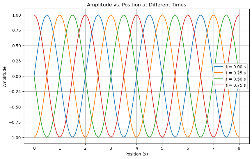
Every location is waving, so here we look at all location at a single time. And then we plot the amplitude of the wave at that location. We can do this for different times.

# Plot amplitude vs. position for different times
times_to_plot = [0, 0.25/f, 0.5/f, 0.75/f]  # Chosen specific times to show one complete cycle

plt.figure(figsize=(10, 6))

for plot_time in times_to_plot:
    plt.plot(x, wave(x, plot_time), label=f't = {plot_time:.2f} s')

plt.title("Amplitude vs. Position at Different Times")
plt.xlabel('Position (x)')
plt.ylabel('Amplitude')
plt.legend()
plt.grid(True)

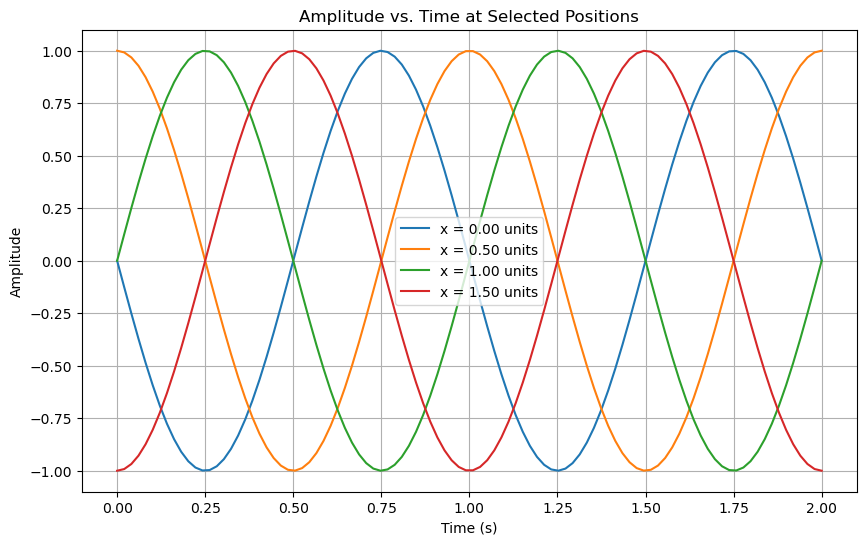
Plotting amplitude vs. time for different positions

At all times the wave is waving, so we can look at the amplitude of the wave at all times for a single location. We can do this for different locations.

# Selected positions to plot
positions_to_plot = [0, lambda_/4, lambda_/2, 3*lambda_/4]

plt.figure(figsize=(10, 6))

for pos in positions_to_plot:
    plt.plot(t, wave(pos, t), label=f'x = {pos:.2f} units')

plt.title("Amplitude vs. Time at Selected Positions")
plt.xlabel('Time (s)')
plt.ylabel('Amplitude')
plt.legend()
plt.grid(True)
plt.show()

Plotting space and time together

It’s a bit hard to see what this 1D wave is doing, so we can instead plot position and time on the plane and let the height represent the amplitude.

# Create a 3D plot
fig = plt.figure(figsize=(12, 8))
ax = fig.add_subplot(111, projection='3d')

ax.plot_surface(X, T, Y, cmap='inferno')  # Using viridis colormap for better clarity
ax.set_title("3D Plot of Traveling Wave in Space and Time")
ax.set_xlabel("Position (x)")
ax.set_ylabel("Time (t)")
ax.set_zlabel("Amplitude")
ax.view_init(elev=30, azim=-60)  # Adjust viewing angle for better visualization

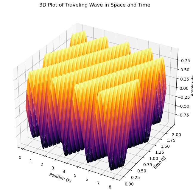
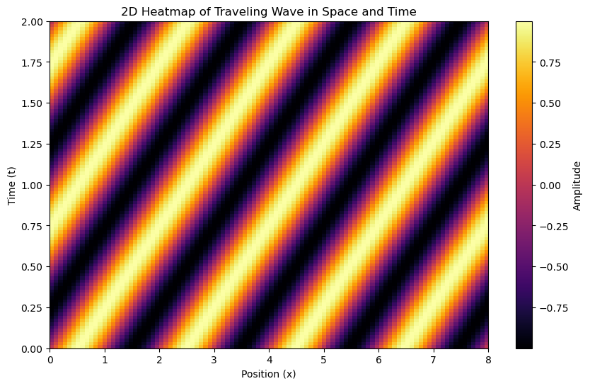
Ok, but make it 2D.

This isn’t the easiest representation to view. You might be able to adjust it a bit with changing the viewing angle. But, we can flatten this plot into a heat map. This is the more common way of viewing these kind of data.

plt.figure(figsize=(10, 6))
plt.imshow(Y, aspect='auto', origin='lower', extent=[x.min(), x.max(), t.min(), t.max()], cmap='inferno')
plt.colorbar(label="Amplitude")
plt.title("2D Heatmap of Traveling Wave in Space and Time")
plt.xlabel("Position (x)")
plt.ylabel("Time (t)")

plt.show()

But I really want to animate it

Sure. Here’s that code.

fig, ax = plt.subplots(figsize=(10, 6))
line, = ax.plot(x, wave(x, 0))  # Initial plot (t=0)
ax.set_ylim([-A, A])  # Setting the y limits to the amplitude range
ax.set_xlabel('Position (x)')
ax.set_ylabel('Amplitude')
ax.grid(True)
ax.set_title("Amplitude vs. Position over Time")

def update(frame):
    line.set_ydata(wave(x, frame))  # Update the y data of the line plot for the current time frame
    ax.set_title(f"Amplitude vs. Position at t = {frame:.2f} s")
    return line,

# Animate over the given times using FuncAnimation
ani = FuncAnimation(fig, update, frames=t, blit=True, interval=50)
plt.close(fig) ## needed to stop another static image from being displayed

# Display the animation in the notebook
HTML(ani.to_jshtml())

Once Loop Reflect

## your code here

## REMEMBER THAT YOU ARE WORKING ON SUPERPOSITION OF WAVES

Implications of Superposition: Diffraction

One of the key indicators of wave like behavior is diffraction. Diffraction is the bending of waves around obstacles and it is a consequence of superposition.

In the case of single-slit diffraction, the wave is diffracted around a slit of width \(a\). a forms circular wave fronts that interfere with each other.

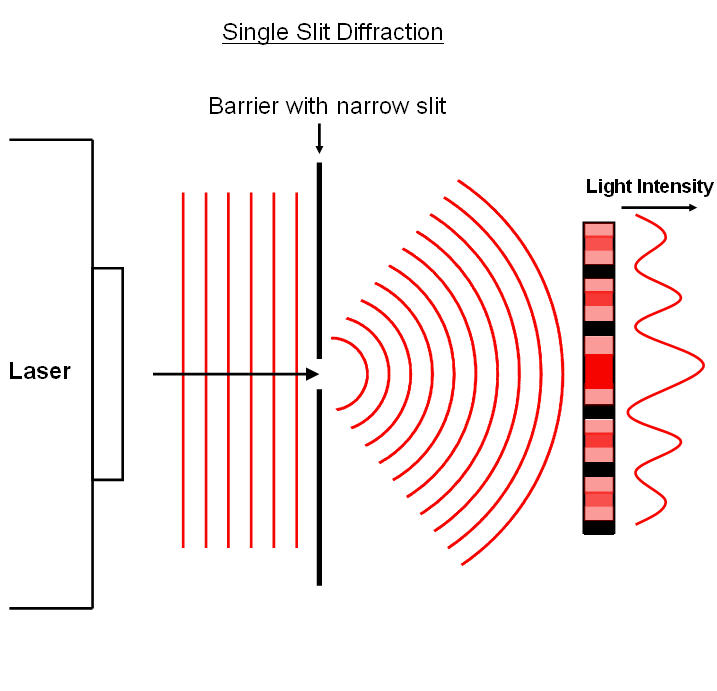
A screen placed a distance \(L\) away from the slit will show a diffraction pattern. We can show the intensity of the diffraction pattern is:

\[I(\theta) = I_0\left(\dfrac{\sin(\beta)}{\beta}\right)^2\]

where

\[\beta = \dfrac{\pi a \sin(\theta)}{\lambda}\]

and \(\lambda\) is the wavelength of the wave and \(\theta\) is the angle of the diffracted wave from the center of the slit (\(\tan(\theta) = y/L\) where \(y\) is the location along the screen).

✅ Do this

1. Plot the intensity of the diffraction pattern for a single slit of width \(a=1\) mm and wavelength \(\lambda=500\) nm.

2. Find the slit width needed to form a diffraction pattern for a typical water wave. You will need to make some estimates.

3. For atomic spacing (\(10^{-10}\) m), use your plotting tool to estimate the wavelength needed to form a diffraction pattern. You will need to make some estimates.

## your code here