Python Basics Review

1. Varables

In python, we use variables to contain data. Here are the most common types:

• Integers: These are exactly what they sound like, they are values that look like \(... ,-3,-2,-1,0,1,2,3,...\).

• Floating Point Numbers: Floats take on Real number values.

• Strings: Strings store text instead of numerical values and are declared within "" or ''.

• Booleans: Bools are either True or False.

a_int = 5
a_float = 1.618
a_str = "Welcome to MSU!"
a_bool = True          # this is a comment, anything after a # is ignored when the code is run
a_complex = 5.0 + 2.4j # complex numbers are in python too, and use j instead of i

# print() lets you output variables, sepearated by commas
print(a_int,a_float,a_str,a_bool,a_complex) 

5 1.618 Welcome to MSU! True (5+2.4j)

Note that when you run a cell, the lines are ran from top to bottom.

type() can be used to find the type of a given variable. Python is a “duck typing” language so it automatically picks the type of any given variable when you declare one with =.

print(type(a_int),type(a_float),type(a_str),type(a_bool),type(a_complex))

<class 'int'> <class 'float'> <class 'str'> <class 'bool'> <class 'complex'>

2. Operators

2.1 Arithmetic

In python we can perform basic arithmetic operations:

a = 4.0
b = 3.5
print(a + b) # Addition
print(a - b) # Subtraction
print(a * b) # Multiplication
print(a / b) # Division
print(a ** b) # Exponentiation

7.5
0.5
14.0
1.1428571428571428
128.0

We could also store these as new variables:

x = 1.1
y = -23.5
z = x**2 + 2*y
print(z)

-45.79

Or update the value of an existing variable:

x = 1.1
x = x + 1.0 # this is the same as x += 1.0
print(x)

2.1

2.2 Comparision

Often it is useful to compare the values of different variables, these comparisions return booleans.

a = 4.0
b = 3.5
print(a == b)
print(a != b)
print(a < b)
print(a > b)
print(a <= b)
print(a >= b)

False
True
False
True
False
True

3. Lists, Tuples, and Dictionaries

3.1 Lists

Lists store several variables. These variables need not be the same type. Lists are declared with [] with commas separating entries.

a_list = [a,b,a_bool,a_str, "another entry", 5]
print(a_list)

[4.0, 3.5, True, 'Welcome to MSU!', 'another entry', 5]

Lists can be indexed with [i] after the name of the list, where i is the index. Note that the first element of a list corresponds to index \(0\).

print(a_list[0], a_list[5],a_list[-1])

4.0 5 5

You can append something to a list, adding a new variable to the end of it:

a_list.append(6)
print(a_list)

[4.0, 3.5, True, 'Welcome to MSU!', 'another entry', 5, 6]

Or change the value of an entry of the list (lists are mutable):

print(a_list)
a_list[2] = False
print(a_list)

[4.0, 3.5, True, 'Welcome to MSU!', 'another entry', 5, 6]
[4.0, 3.5, False, 'Welcome to MSU!', 'another entry', 5, 6]

We can also find the length of a list with len. Note that len starts counting at one:

print(len([]))
print(len(a_list))

0
7

3.2 Tuples

There is another object similar to lists called tuples. We can create tuples using (), and index them just like lists:

a_tuple = (1,2,3,4) # initialize like a list, but with () instead of []
# note that tuples don't require the parenthesis, we could have written a_tuple = 1,2,3,4
print(a_tuple)
print(a_tuple[0])

(1, 2, 3, 4)
1

However, unlike lists, tuples are not mutable, which means that you can’t change the value of any of the values in the tuple. So the following code would not work.

a_tuple = (1,2,3,4)
a_tuple[0] = 2 # this line is not allowed

Tuples are more memory efficient than lists.

Another useful thing that can be done with tuples is they can be unpacked. This means you can take a tuple and save each of it’s entries as a different variable. Here is an example of unpackig a tuple:

a_tuple = (1,2,3,4)
a,b,c,d = a_tuple
print(a,b,c,d)

1 2 3 4

This can be done with lists as well:

a_list = [1,2,3,4]
a,b,c,d = a_list
print(a,b,c,d)

1 2 3 4

3.3 Dictionaries

Dictionaries store values in key:value pairs.

a_dict = {
  "name": "Danny",
  "department": "Physics and Astronomy",
  "simultaneous meetings": 512
}
print(a_dict)

{'name': 'Danny', 'department': 'Physics and Astronomy', 'simultaneous meetings': 512}

These can be indexed with the keys:

print(a_dict['department'])

Physics and Astronomy

You can directly obtain the keys of a dictionary with .keys()

print(a_dict.keys())

dict_keys(['name', 'department', 'simultaneous meetings'])

4. Arrays

NumPy Arrays store many floating point numbers (or complex numbers). These are part of the python library NumPy which is probably the most important python library.

import numpy as np # import numpy

a_ary = np.array([0.0,2.1,-2.0,6.18])
print(a_ary)

print(a_ary[0]) # arrays are indexed like lists

[ 0.    2.1  -2.    6.18]
0.0

One great thing about numpy arrays is that it is easy to perform mathematical operations on the whole array:

print(a_ary + 1)
print(2 * a_ary)

[ 1.    3.1  -1.    7.18]
[ 0.    4.2  -4.   12.36]

Multi-Dimensional Arrays can also be made:

a_ary = np.array([[1,2],[3,4]])

print(a_ary)
print(a_ary[0,0],a_ary[0,1]) # multi dimensional indexing

[[1 2]
 [3 4]]
1 2

In the case of 2d arrays, we can also perform matrix multiplication with @:

b_ary = np.array([[5,6],[7,8]])

print(a_ary@b_ary) # multiply matrices

[[19 22]
 [43 50]]

Often you might need to generate arrays of certain values. np.linspace and np.arange give two ways of making arrays with values that span a range:

x1 = np.linspace(0,1,11)  # 11 evenly spaced numbers from 0 to 1
x2 = np.arange(0,1.1,0.1) # numbers from 0 to 1 with spacing 0.1
print(x1)
print(x2)

[0.  0.1 0.2 0.3 0.4 0.5 0.6 0.7 0.8 0.9 1. ]
[0.  0.1 0.2 0.3 0.4 0.5 0.6 0.7 0.8 0.9 1. ]

np.zeros and np.ones give ways to generate arrays of just zeroes or ones:

x3 = np.zeros(5)
x4 = np.ones((2,3))
print(x3)
print(x4)

[0. 0. 0. 0. 0.]
[[1. 1. 1.]
 [1. 1. 1.]]

You can use len for 1d arrays just like you would for lists, but .shape is often more useful, especially for multi-dimensional arrays:

print(len(x3))
print(x3.shape)
print(x4.shape)

5
(5,)
(2, 3)

You can also perform boolean masks which let you use conditional logic on an array to select for certain values:

x = np.arange(-2,2.5,0.5) # values from -2 to 2 in step size of 0.5

x_mask = x >= 0 # mask for only positive values
print('mask:', x_mask)

x_masked = x[x_mask] # apply the mask to the original array
print("masked:",x_masked)

mask: [False False False False  True  True  True  True  True]
masked: [0.  0.5 1.  1.5 2. ]

Note that we could have done this masking in just one line:

print(x[x >= 0])

[0.  0.5 1.  1.5 2. ]

Numpy has a wealth of other functionality, such as built in functions like sin or exp or methods for arrays such as finding the maximum of an array with .max or the index of that entry with .argmax, but there are far too many of these methods to list here. NumPy even has a fast fourier transform! A general rule of thumb is if you think it would exist, it probably does and you can find it in the numpy documentation.

5. Plotting

One of the great things about python is that it makes plotting pretty simple, thanks to the matplotlib library.

import matplotlib.pyplot as plt # import matplotlib

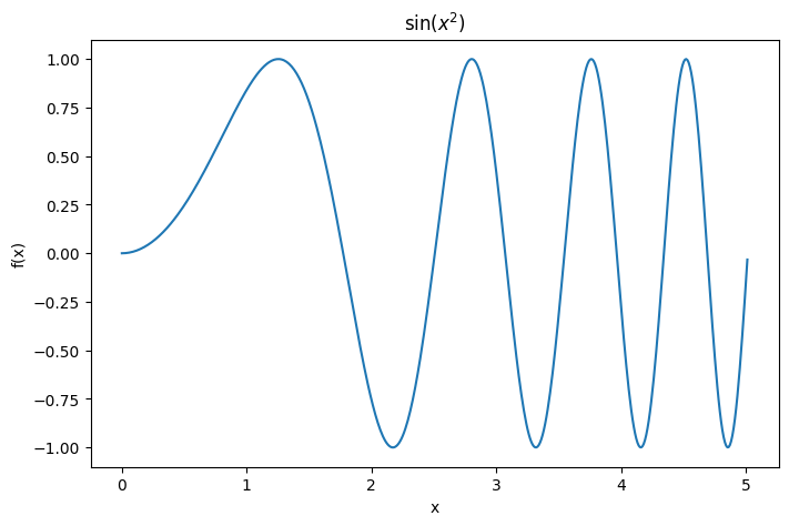
The most basic kind of plotting with matplotlib uses plt.plot. For example, lets say you want to plot the function: \(\sin(x^2)\). That can be done like this:

x = np.arange(0,2*np.sqrt(2*np.pi),0.01) # set up x array
y = np.sin(x**2)

plt.figure(figsize=(8,5))
plt.plot(x,y)
plt.title(r"$\sin(x^2)$") # r strings let you use latex in plots
plt.xlabel('x')
plt.ylabel('f(x)')
plt.show()

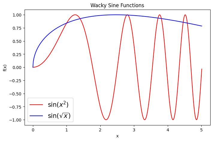
You can also plot multiple things on the same plot by using plt.plot twice:

x = np.arange(0,2*np.sqrt(2*np.pi),0.01) # set up x array
y = np.sin(x**2)
y2 = np.sin(np.sqrt(x))

plt.figure(figsize=(8,5))
plt.plot(x,y, label = r"$\sin(x^2)$", c = 'r') # now additionally specifying the label for the legend as well as the color of the plot
plt.plot(x,y2, label = r"$\sin(\sqrt{x})$", c = 'b')
plt.title("Wacky Sine Functions")
plt.xlabel('x')
plt.ylabel('f(x)')
plt.legend(fontsize = 15)
plt.show()

Matplotlib has tons of other features as well, such as scatter plots, bar charts, subplots and 3d plotting, just to name a few. This article has a lot of great information on getting started with matplotlib.

6. Loops

Sometimes you need to be able to write an algorithm yourself. To do this, we use loops. Specifically, there are two main kinds of loops, for loops and while loops.

6.1 For Loops

For looops loop over a container. They have the form for x in y: where y is the container. As the loop runs, x takes on the value of everything stored in y, one after the other. Lines of code that are part of the loop after its declaration must be indented in the lines after the loop is declared. Here are a couple examples of simple for loops:

a_list = [4,5,'six','seven']

print('loop 1:')
for item in a_list:
    print(item)

print('loop 2:')
for i in range(1,5): # range(a,b) is a range of integers from a to b-1
    print(i)

loop 1:
4
5
six
seven
loop 2:
1
2
3
4

6.2 While Loops

While loops continue to run while some logical statement is True and stop running when that statement is False.

a = 4
b = 0
while a > 0 and b < 10: # you can use "or" and "and" to put multiple boolean statements together
    a -= 1
    b += 1
    print('a:',a,'b:',b)

a: 3 b: 1
a: 2 b: 2
a: 1 b: 3
a: 0 b: 4

A warning - If you make a mistake when using while loops, it is much easier for things to go spectacularly wrong since a loop could try to run forever. A good general rule of thumb is to use for loops whenever possible and only use while loops when it is extremely convienient to do so.

5.3 Example: Numerical Integration of Object Falling in 1d

When learning loops in python, it can be useful to see how you would do the same thing a couple different ways. Here, we show two ways of numerically solving an object falling in 1d with no air resistance. We choose \(m = 1 kg\), \(v_0 = 0 m/s\), \(p_0 = 0 kgm/s\), and \(y_0 = 500 m\) for initial conditions and the standard \(g = 9.81 m/s^2\) for the acceleration due to gravity.

The numerical method we are going to use is called Euler’s Method, which is the simplest but also least effective numerical integration technique. Euler’s method works by first updating the momentum of the object with the force it feels, then it updates the position of the object using its velocity (which can be found from \(v = p/m\)).

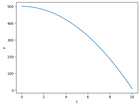
First we’ll show a way of doing this using a for loop and numpy array indexing, and we’ll plot the results:

# time and array setup
dt = 0.01  # time step [s]
t = np.arange(0,10,dt) # time array [s]
y = np.zeros(len(t))   # position array (starts as just zeros) [m]
p = np.zeros(len(t))   # momentum array (starts as just zeros) [kg*m/s]

# parameters and initial conditions
g = -9.81  # acceleartion due to gravity [m/s**2]
m = 1      # mass [kg]
y0 = 500   # initial position [m]
y[0] = y0  # set initial position in position array [m]
p0 = 0     # initial momentum [kg*m/s]
p[0] = p0  # set initial momentum in momentum array [kg*m/s]


for i in range(len(t)-1): # range starts at 0 when only one value is specified
    p[i+1] = p[i] + m * g * dt    # calculate the next momentum according to dp = F*dt
    y[i+1] = y[i] + (p[i]/m) * dt # calculate the next position according to dy = V*dt

plt.plot(t,y)
plt.xlabel('t')
plt.ylabel('y')
plt.show()

Next, here is a way to do this using a while loop and lists:

# time setup
dt = 0.01
t = 0     # initial time [s]
tf = 10   # final time   [s]

# parameters and initial conditions
g = -9.81 
m = 1
y = 500  # initial position [s]
p = 0    # initial momentum [s]

# lists to store values
t_list = [0]
y_list = [y]

while t < tf:
    p += m * g * dt
    y += (p/m) * dt
    y_list.append(y) # append new value of y to y_list
    t += dt
    t_list.append(t) # append new value of t to t_list

plt.plot(t_list,y_list)
plt.xlabel('t')
plt.ylabel('y')
plt.show()

6.4 if and else statements

Conditional logic in loops is often very useful. This can be done with if and else statements. Here’s an example:

for number in np.arange(1,5):
    if number % 2 == 0: # Check to see if number is even
        print(number, "is even")
    else: 
        print(number, "is odd")

1 is odd
2 is even
3 is odd
4 is even

You can include multiple conditions by using elif:

for number in np.arange(1,7):
    if number % 3 == 0 and number % 2 ==0:
        print(number,'is even and divisible by 3')
    elif number % 3 == 0:
        print(number, "is divisible by 3")
    elif number % 2 == 0:
        print(number, "is even")
    else: 
        print(number, "is odd")

1 is odd
2 is even
3 is divisible by 3
4 is even
5 is odd
6 is even and divisible by 3

6.5 Nested loops

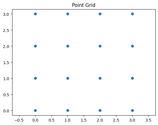
multiple loops can be nested within each other. Here’s an example of a code that makes a grid of points and plots them.

x = 0
y = 0
x_list = []
y_list = []
size = 4
step = 1

for x in range(size):
    for y in range(size): # loop over y values for each x value
        x_list.append(x)
        y_list.append(y)

plt.scatter(x_list,y_list)
plt.title('Point Grid')
plt.axis('equal')
plt.show()

7. Functions

Often you may want to repeat a calculation in python many times. Functions are super useful for this. Functions are declared with def functionname(imputs): and will return anything after the word return is used. Here’s an example of a simple function that calculates the square root of a number:

def sqrt(x):
    return x**0.5

print(sqrt(4))

2.0

Functions can have as many imputs and outputs as you want and can be as complicated as you’d like. For example, we could turn the numerical integration example from earlier into a function:

def falling_object(dt,t,y,p,y0=500,p0=0,m = 1,g = -9.81): # variables can be set to default values when the function is defined

    y[0] = y0
    p[0] = p0

    for i in range(len(t)-1):
        p[i+1] = p[i] + m * g * dt    
        y[i+1] = y[i] + (p[i]/m) * dt 

    return y,p

dt = 0.01  # time step [s]
t = np.arange(0,10,dt) # time array [s]
y = np.zeros(len(t))   # position array (starts as just zeros) [m]
p = np.zeros(len(t))   # momentum array (starts as just zeros) [kg*m/s]

y,p = falling_object(dt,t,y,p) # call the function

plt.plot(t,y)
plt.xlabel('t')
plt.ylabel('y')
plt.show()

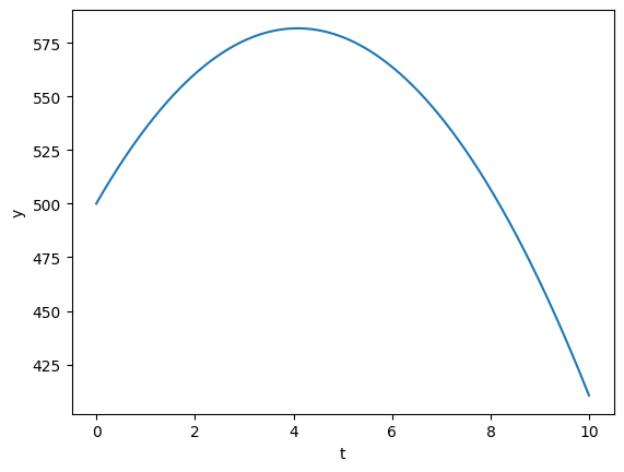
Note that having this as a function makes it really easy to try different initial conditions, since all we have to do is change the imput to the function:

y,p = falling_object(dt,t,y,p, p0 = 40)

plt.plot(t,y)
plt.xlabel('t')
plt.ylabel('y')
plt.show()