Support Vector Machines (Radial Kernel)

• As a classifier, an SVM creates new dimensions from the original data, to be able to seperate the groups along the original features as well as any created dimensions.

• The kernel that we choose tells us what constructed dimensions are available to us.

• We will start with a linear kernel, which tries to construct hyper-planes to seperate the data.

  • For 2D, linearly separable data, this is just a line.

• We are now going to use a new kernel: RBF, this will create new dimensions that aren’t linear. You do not need to know the details of how this works (that is for later coursework).

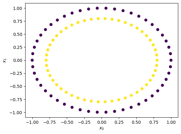
We use make_circles because it gives us control over the data and it’s separation; we don’t have to clean or standardize it.

Let’s make some circles

##imports
import numpy as np
import matplotlib.pyplot as plt
from mpl_toolkits.mplot3d import Axes3D
from sklearn.datasets import make_circles
from sklearn.svm import SVC
from sklearn.model_selection import train_test_split
from sklearn.metrics import classification_report, confusion_matrix, roc_curve, roc_auc_score

X,y = make_circles(n_samples = 100, random_state = 3)

## Plot Circles
plt.scatter(X[:,0], X[:,1], c=y)
plt.xlabel(r'$x_0$'); plt.ylabel(r'$x_1$')

Text(0, 0.5, '$x_1$')

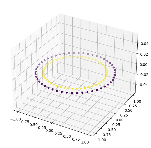
Let’s look at the data in 3D

fig = plt.figure(figsize = (10, 7))
ax = plt.axes(projection ="3d")

ax.scatter3D(X[:,0], X[:,1], 0, c=y)

<mpl_toolkits.mplot3d.art3d.Path3DCollection at 0x13fb1f4a0>

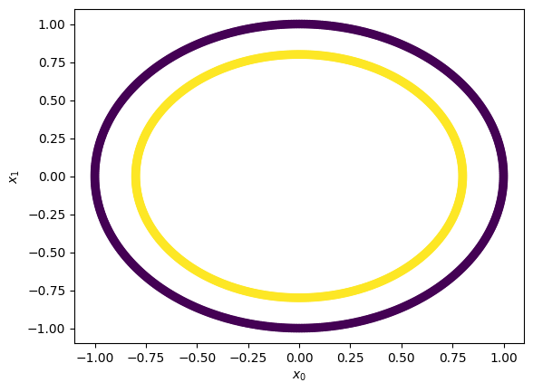
Let’s make a little more data

X,y = make_circles(n_samples = 1000, random_state = 3)

## Plot Blobs
plt.scatter(X[:,0], X[:,1], c=y)
plt.xlabel(r'$x_0$'); plt.ylabel(r'$x_1$')

Text(0, 0.5, '$x_1$')

Let’s train up a linear SVM

• This is what we did last class; but now we have split the data

## Split the data
train_vectors, test_vectors, train_labels, test_labels = train_test_split(X, y, test_size=0.25)

## Fit with a linear kernel
cls = SVC(kernel="linear", C=10)
cls.fit(train_vectors,train_labels)

## Print the accuracy
print('Accuracy: ', cls.score(test_vectors, test_labels))

Accuracy:  0.444

Let’s check the report and confusion matrix

• We want more details than simply accuracy

## Use the model to predict
y_pred = cls.predict(test_vectors)

print("Classification Report:\n", classification_report(test_labels, y_pred))

print("Confusion Matrix:\n", confusion_matrix(test_labels, y_pred))

Classification Report:
               precision    recall  f1-score   support

           0       0.47      0.38      0.42       133
           1       0.42      0.52      0.47       117

    accuracy                           0.44       250
   macro avg       0.45      0.45      0.44       250
weighted avg       0.45      0.44      0.44       250

Confusion Matrix:
 [[50 83]
 [56 61]]

Let’s look at the ROC curve and compute the AUC

## Construct the ROC and the AUC
fpr, tpr, thresholds = roc_curve(test_labels, y_pred)
auc = np.round(roc_auc_score(test_labels, y_pred),3)

plt.plot(fpr,tpr)
plt.plot([0,1],[0,1], 'k--')
plt.xlabel('FPR'); plt.ylabel('TPR'); plt.text(0.6,0.2, "AUC:"+str(auc));

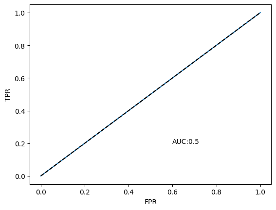
The Linear Kernel Absolutely Failed!

Let’s use RBF instead and see what happens

1. Train the model

2. Test the model

3. Evalaute the model: accuracy, scores, confusion matrix, ROC, AUC

Train the model and start evaluating it

## Fit with a RBF kernel
cls_rbf = SVC(kernel="rbf", C=10)
cls_rbf.fit(train_vectors,train_labels)

## Print the accuracy
print('Accuracy: ', cls_rbf.score(test_vectors, test_labels))

Accuracy:  1.0

Use the model to predict and report out

## Use the model to predict
y_pred = cls_rbf.predict(test_vectors)

print("Classification Report:\n", classification_report(test_labels, y_pred))

print("Confusion Matrix:\n", confusion_matrix(test_labels, y_pred))

Classification Report:
               precision    recall  f1-score   support

           0       1.00      1.00      1.00       133
           1       1.00      1.00      1.00       117

    accuracy                           1.00       250
   macro avg       1.00      1.00      1.00       250
weighted avg       1.00      1.00      1.00       250

Confusion Matrix:
 [[133   0]
 [  0 117]]

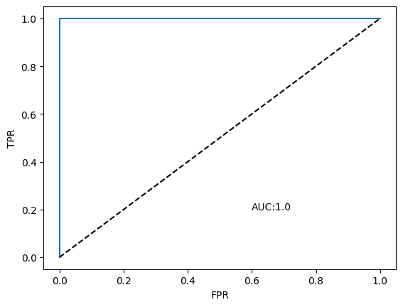
Construct the ROC and the AUC

## Construct the ROC and the AUC
fpr, tpr, thresholds = roc_curve(test_labels, y_pred)
auc = np.round(roc_auc_score(test_labels, y_pred),3)

plt.plot(fpr,tpr)
plt.plot([0,1],[0,1], 'k--')
plt.xlabel('FPR'); plt.ylabel('TPR'); plt.text(0.6,0.2, "AUC:"+str(auc));

Today

• We are going to use SVM with real data. We are going to use the linear kernel again, but you can change to RBF (it will take much longer to run).

• We are also going to introduce hyper-parameter optimization and grid searching (again takes more time)

In the construction of the SVM: cls = svm.SVC(kernel="linear", C=10), C is a hyperparameter that we can adjust. sklearn has a mechanism to do this automatically via a search and find the “best” choice: GridSearchCV.

Please ask lots of questions about what the code is doing today because you are not writing a lot of code today!

Questions, Comments, Concerns?