Day 15 - Potential Energy and Stability

Infinite Potential Well \(\longrightarrow\)

---

Infinite Potential Well

\[\begin{split}V(x) = \begin{cases} 0 & 0 < x < L \\ \infty & \text{otherwise} \end{cases}\end{split}\]

Classical Motion in an Infinite Potential Well

Particle bounces back and forth between the walls of the well with constant speed.

Quantum Motion in an Infinite Potential Well

Particle has quantized energy levels and corresponding wavefunctions that are sinusoidal within the well and zero outside the well.

---

Announcements

• Midterm 1 is available (Due 27 Feb; late 1 Mar)

  • You may work in larger groups, but solutions are submitted like homework (max 3 group members) on Gradescope

  • Exercise 0 is for project planning; and can be submitted individually or as a different group on D2l

• Friday’s Class: Work period for Midterm 1; you can ask us questions and check in on your progress.

---

Midterm 1 - Exercise 0

Can be completed individually or as a group (different from your homework/midterm group)

• Read about Computational Essays

  • Respond to two questions (~200 words each) about your readings.

• Think about the topic and research question you want to explore for your project

  • All together, write about ~500 words describing your project idea.

Submitting on D2L because DC will give you feedback on your project idea.

---

Midterm 1 - Exercise 1

Modeling Spin Dependent Forces

\[\mathbf{F}_{magnus} = S \mathbf{\omega} \times \mathbf{v}\]

• The next complication beyond air drag

• You may use prior codes or solutions from homework, but you must modify them to include the Magnus force.

• The model should be of your own choosing (i.e., your choice of sports ball)

Submit on Gradescope (including PDF of Jupyter notebook).

What you are learning: How to model a new situation that is just a little more complicated than what we’ve done before.

---

Midterm 1 - Exercise 2

Particle in a one-dimensional potential

\[V(x) = \frac{V_0}{d^4}(x^4 - 2x^2d^2+d^4)\]

• Complete a full analysis of the potential using all tools we have learned so far

• Demonstrate your understanding of the potential by modeling motion of a particle

Submit on Gradescope (including PDF of Jupyter notebook).

What you are learning: How to analyze a new potential energy function based on the theoretical tools and computational tools we have learned so far.

---

Midterm 1 - Exercise 3

Model your own system

\[V(x) = ?\]

• Choose a 1D potential energy function that you find interesting

• Analyze the potential energy function using all tools we have learned so far

• Model the motion of a particle in this potential energy function

Submit on Gradescope (including PDF of Jupyter notebook).

What you are learning: Taking agency over your learning by applying what you have been scaffolded to learn to a system of your own choosing.

---

Reminders: Finding Equilibrium Points

Given a potential energy function \(U(x)\), we can find the equilibrium points by setting the derivative of the potential energy function to zero:

\[\frac{dU(x^*)}{dx} = 0.\]

The stability of the equilibrium points can be determined by examining the second derivative of the potential energy function:

\[\frac{d^2U(x^*)}{dx^2}>0? \qquad \frac{d^2U(x^*)}{dx^2}<0?\]

If the second derivative is positive, the equilibrium point is stable. If the second derivative is negative, the equilibrium point is unstable.

---

Clicker Question 15-1

Here’s the graph of the potential energy function \(U(x)\) for a pendulum.

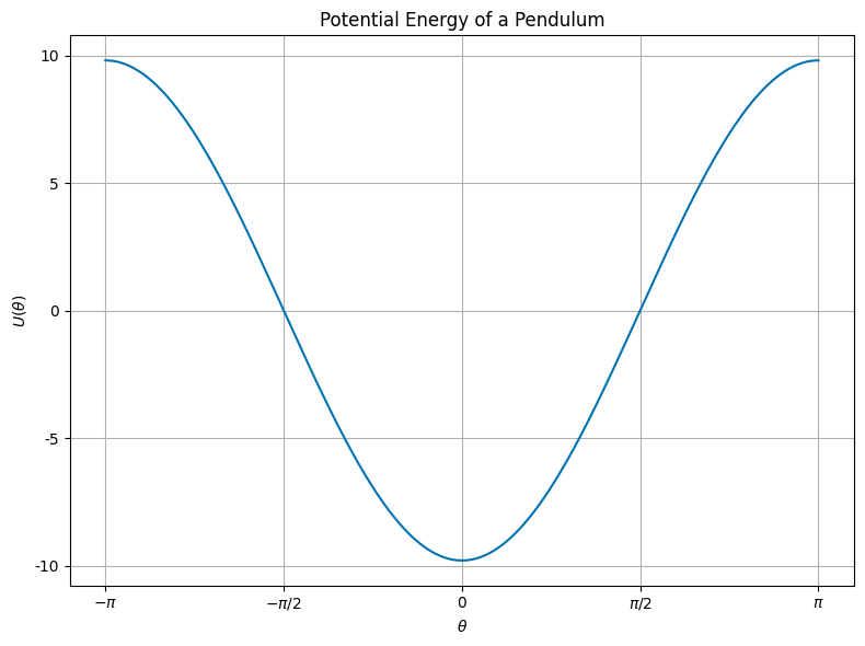
What can you say about the equilibrium points? There is/are:

1. One stable point

2. Two stable points

3. One stable and one unstable point

4. Two unstable and one stable point

---

Clicker Question 15-2 (similar to Midterm 1 Exercise 2)

A double-well potential energy function \(U(x)\) is given by

\[U(x) = -\frac{1}{2}kx^2 + \frac{1}{4}kx^4.\]

We assume we have scaled the potential energy so that all the units are consistent.

How many equilibrium points does this system have?

1. 1

2. 2

3. 3

4. 4

---

Clicker Question 15-3

A double-well potential energy function \(U(x)\) is given by

\[U(x) = -\frac{1}{2}kx^2 + \frac{1}{4}kx^4.\]

1. Find the equilibrium points (\(x^*\)) of the pendulum by setting:

\[\frac{dU(x^*)}{dx} = 0.\]

2. Characterize the stability of the equilibrium points (\(x^*\)):

\[\frac{d^2U(x^*)}{dx^2}>0? \qquad \frac{d^2U(x^*)}{dx^2}<0?\]

Click when done.

---

Clicker Question 15-4

Here’s a graph of the potential energy function \(U(x)\) for a double-well potential.

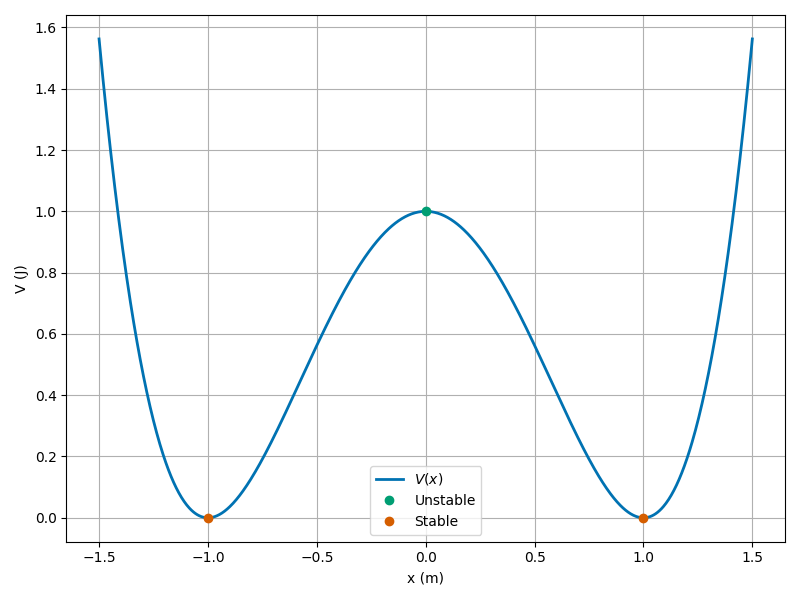
Describe the motion of a particle with the total energy, \(E=\)

1. \(0.4\,\mathrm{J}\), \(<\) barrier height

2. \(1.2\,\mathrm{J}\), \(>\) barrier height

3. \(1.0\,\mathrm{J}\), \(=\) barrier height

Click when done.

---

Clicker Question 15-5

Here’s the graph of the potential energy function \(V(x)\) that is a model of quark confinement in quantum chromodynamics.

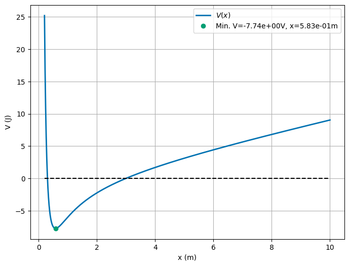
What can you say about the equilibrium points? There is/are:

1. One stable point

2. One stable and one unstable point

3. Can’t tell

---

Clicker Question 15-6

Here’s the equation for this potential energy function (constants: \(\gamma\), \(\delta\), and \(\kappa\)):

\[V(v) = -\frac{\gamma}{x} + \frac{\delta}{x^2} + \kappa x,\]

What can you say about the motion of a particle with energy \(E\)?

1. \(E < 0\) \(\;\) 2. \(E = 0\) \(\;\) 3. \(E > 15\)

Careful with #3! Send \(x\) to \(\infty\): \(\lim_{x\to\infty} V(x) = ?\)