
05 - Conservation Laws Govern and Constrain our Physics#
![]()
Handwritten Notes
Learning Goals#
After studying Lesson 05, you should be able to:
Predict the conditions under which the total energy of a system remains constant using the principle of energy conservation.
Differentiate between various forms of energy (e.g., kinetic, potential, internal) and describe their transformations within a system.
Analyze the role of energy conservation in systems with external forces and quantify energy changes throughout a process.
Apply the concept of a point particle to simplify energy calculations and understand its limitations in modeling real-world systems.
Predict the conditions under which the total linear and angular momentum of a system remain constant using conservation laws.
Derive and apply the discrete update equations for linear and angular momentum in systems with external forces.
We started with Newton’s Laws of Motion because they provide a framework for us to develop the equations of motion. However, there is a broader framework that can help us understand and organize our knowledge of physics. These are conservation laws.
Conservation laws are principles that state that certain properties of a system remain constant over time. These properties are called conserved quantities. In classical mechanics, there are three main conservation laws:
Conservation of Energy: The total energy of an isolated system remains constant over time.
Conservation of Momentum: The total momentum of an isolated system remains constant over time.
Conservation of Angular Momentum: The total angular momentum of an isolated system remains constant over time.
We will discuss them briefly below, before we dive into the details of conservation of energy. The concept of energy is so important and complimentary to our understanding of motion that we will focus on it before returning to momentum and angular momentum.
What is Energy?#
Energy is a central concept of science. It is also a very challenging conceptual idea. Physicists are known to say things like,
“I can’t tell you what energy is, but I can tell you how to calculate it.”
Richard Feynman is known to have had a disdain for the wildly different units of energy that we use in physics.
Feynman on the units of energy (2 minute video)
Feynman is quoted as saying:
“It is important to realize that in physics today, we have no knowledge of what energy is.”
Energy is a number, a quantity, that when we compute it, we find it stays the same before and after a process - so long as we account for all the interactions and uses in that case.
Conservation of energy states that there is not temporal change in the total energy of a system. This is a very powerful idea, but it is not always easy to apply.
If this equation holds between any two states of a system, we say that energy is conserved. A simpler statement is thus,
Energy is a challenging concept#
To frame how interesting and complex energy can be, consider this video from Veritasium:
How do we get light from a circuit when we close a switch? (14 minute video)
There a many potential forms of energy and lots of processes that convert energy from one form to another. Below is a table of some common forms in physics. In addition, we have listed subsets of these forms that are often useful to distinguish. We will do analyses that include most of these forms.
Main Form of Energy |
Narrower Distinction |
Description |
|---|---|---|
Kinetic Energy |
Energy of macroscopic motion |
|
Translational |
Energy due to point particle translation |
|
Rotational |
Energy due to rotation |
|
Vibrational |
Energy due to vibration |
|
Potential Energy |
Energy due to position |
|
Gravitational |
Energy due to position in a gravitational field |
|
Elastic |
Energy due to deformation of an elastic object |
|
Electric |
Energy due to position in an electric field |
|
Internal Energy |
Energy due to microscopic motion |
The Point Particle#
Critical to the understanding of energy is that it is a property of a system. A system can consist of a single object or be made of many different objects. In the case of modeling the motion of a single object, we often introduce the concept of a point mass or point particle. A point mass is an idealized object that has mass but no size or shape. It has no internal structure and thus no internal energy. It is a useful abstraction for modeling the motion of objects in classical mechanics.
Point Particle and Real Models (6 minute video)
The video below is from an introductory physics course at Georgia Tech. It covers the important aspects of a point particle and how we miss some of the details when we focus exclusively on the point particle model.
Some YouTube videos are unable to be embedded in Jupyter Books. Click the image below to watch the video on YouTube.

Kinetic Energy of a Point Mass#
In that case of a point particle, we often focus on the kinetic energy of the object. The classical kinetic energy of a point mass is given by the equation:
where \(m\) is the mass of the object and \(v\) is its velocity. The kinetic energy of a point mass is a scalar quantity, which as we will learn is much easier to work with than a vector quantity.
However, we can loose some information by moving to an energy-only framework; we typically focus on the behavior before and after a process and not the details of the process itself when using energy conservation.
Work#
Work is a concept closely related to energy, it describes the transfer of energy from one system to another. Our definition of work is macroscopic and thus will not related to temperature. Increases in temperature are related to internal energy, and thus the micrscopic motion of the particles in a system. As we consider a point particle moving from one location to another under a given force, we can define the work done by that force as:
where \(F(x)\) is the one-dimensional force acting on the particle between locations \(x_i\) and \(x_f\). More generally, if there is a position dependent force, we can write the work done by that force as:
where \(C\) is the path taken by the particle and \(d\vec{l}\) is a differential displacement vector along that path.
Work-Energy Theorem#
The work-energy theorem show the relationship between work and the change in kinetic energy of a point mass. The work done on a point mass is equal to the change in its kinetic energy:
Conservation of Momentum and Angular Momentum#
Linear Momentum is a vector quantity that describes the motion of an object. It is defined as the product of an object’s mass and its velocity:
Angular Momentum is a vector quantity that describes the rotational motion of an object. It is defined as the cross product of the position vector and the momentum vector:
These two other conservation laws are vector conservation laws. That is, they hold in each direction. Much like the definition of conservation of energy, we can start with the time derivatives of both momentum and angular momentum.
As before, we can take small steps in time and write the change in momentum and angular momentum as:
And thus, we see that each component is conserved. For momentum,
If the linear momentum is conserved in each direction, then the total linear momentum is conserved. The linear momentum will be the same before and after a process. For angular momentum, we find,
If the angular momentum is conserved in each direction, then the total angular momentum is conserved. The angular momentum will be the same before and after a process.
After we get a handle on energy, we will return to momentum and angular momentum.
Conservation of Energy#
One expression of a conservation law is the conservation of energy. For an isolated and closed system, the total energy is conserved. That is, before and after any process, we can account for all the energy in the system and it is the same. More generally, conservation of energy accounts for the energy “lost” to the surroundings. All of the changes to the system must be accounted for in changes the surroundings.
For a given choice of system that interacts with its surroundings, the change in energy of the system is equal to the work done on the system and any heat exchanged with the surroundings. This is a statement of the first law of thermodynamics. We can write that statement mathematically as:
where \(\Delta E_{\text{system}}\) is the change in energy of the system, \(W\) is the work done on the system, and \(Q\) is the heat exchanged with the surroundings.
Sign conventions
Note that the signs of the work done and heat exchanged are important. But we can remember them by asking if the system is going to increase its energy.
If we add energy into the system by heating it, then \(Q\) is positive because \(\Delta E_{\text{system}}\) is positive. If the remove energy from the system through an exchange of heat, then \(Q\) is negative.
If the system does work on the surroundings, for example, by exerting a force on an external object over some displacement, then \(W\) is negative because \(\Delta E_{\text{system}}\) is negative. If instead the surroundings do work on the system, then \(W\) is positive.
We can rewrite this energy equation as an update equation for the energy of the system:
From this equation, we can see that the final state of the system’s energy is determined by the sum of its initial energy, the work done on the system, and the heat exchanged with the surroundings.
The Work-Energy Theorem#
We often model a system as a single object that interacts with its surroundings. In this case, it’s often beneficial to select the object alone to be the system of interest. Then all of our work is to explain and predict the dynamics of the object.
This simplification allows us to employ a more specialized case of the general energy equation. We can write the work-energy theorem as:
where \(\Delta E_{\text{object}}\) is the change in energy of the object and \(W_{\text{net}}\) is the net work done on the object.
More specifically, we often focus only on the changes to the object’s motion. This is because we use often use the model of a point particle to describe the object. In this case, the object has no internal structure and thus no internal energy. The only energy we need to consider is the object’s kinetic energy, \(K\).
Limitation of this model
The point particle model where we focus on the kinetic energy of an object is an obvious simplification. But it might not be so obvious how quickly it is to break down.
Consider pushing a block across the floor. The block is a point particle and we model it as such. It comes to a stop and we argue the block’s kinetic energy was converted to heat in the floor.
But what about the block itself? Would it’s surface temperature increase? It does, but we don’t account for it.
A great account of these kinds of situations is from my colleague Bruce Sherwood. Bruce’s paper, Pseudowork and real work, American Journal of Physics (1982), is an important read about the limitation of the point particle model. You can find a PDF copy here.
Kinetic Energy#
Our model of kinetic energy stems from a series of experiments dropping stones into clay. The depth of the hole made was proportional to the square of the impact speed.
Through many additional experiments we have quantified the kinetic energy of a point particle as:
We also use \(T\) to represent kinetic energy, so you might see it written as:
Note that this description of the kinetic energy is fully classical. It is the energy of motion in the limit that object moves much slower than the speed of light. We learned from Einstein’s special theory of relativity that the total energy of an point particle is:
where \(\gamma\) is the Lorentz factor and \(c\) is the speed of light. The Lorentz factor is defined as:
Notice that if \(v/c =0\) then,
We call this the “rest energy” of the object. It is the energy of the object when it is not moving, and it demonstrates the mass-energy equivalence.
The remaining energy of the object is the kinetic energy, \(T\). We can write that as:
We can take the limit that \(v/c \ll 1\) and expand the Lorentz factor in a Taylor series to find that:
Then we find that the kinetic energy is:
We have recovered the classical expression for kinetic energy. The higher order terms in the expansion are negligible when \(v/c \ll 1\).
Developing the Work-Energy Theorem#
Let’s start with our definition of the classical kinetic energy of a point particle:
We ask how does \(T\) change with time? We take the time derivative of \(T\):
The last term can be combined because the dot product is commutative. We can factor out the \(m/2\) and write:
Ok, in that expression is the net force on the object,
So that,
Now let’s discretize the time derivative to make sense of this.
That last term is the displacement of the object, \(\Delta \vec{x} = \vec{v}\Delta t\). So we can write:
This is the work done on the object by the net force. We can write that as:
Overall Effect of the Forces#
Consider that we are looking at the changes in the object’s motion over a longer period of space and time. This discrete model above helps us understand the relationship between the work done on the object and the change in its kinetic energy in a small interval, but what about the overall effect of the forces on the object?
Consider a discrete set of \(n\) spatial intervals, \(\Delta x_i\), where \(i\) is the index of the interval.
At each of these spatial intervals, we experience a different net force, like in the figure below.
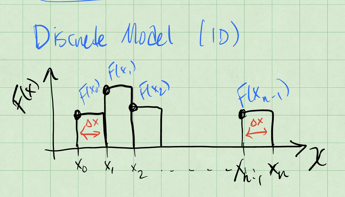
Fig. 19 A discrete force model.#
Error
Redraw as vector graphic and post SVG
The work done by this force is the change in kinetic energy of the object:
Notice that in the limit that \(n \rightarrow \infty\) and \(\Delta x_i \rightarrow 0\), we have a continuous function of the net force. We can write that as:
Thus, in our continuous limit, we can write the work done by the net force as:
What about in more than one dimension?
Work done in more than one dimension#
Consider a path \(C\) that we have discretized into \(n\) intervals. The object starts at \(\vec{r}_0\) and ends at \(\vec{r}_n\). Each interval is \(\Delta \vec{r}_i\) and the net force is \(\vec{F}_{net,i}\). The figure below shows the work done by the net force in each interval.
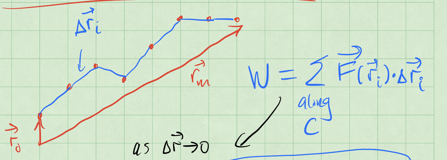
Fig. 20 Work done by a discrete net force along a path.#
Error
Redraw as vector graphic and post SVG
The work done by the net force is:
as \(\Delta \vec{r}_i \rightarrow 0\) and \(n \rightarrow \infty\), we have a continuous function of the net force. We can write that as:
The work can be positive, if the force and displacement are in the same direction, or negative, if they are in opposite directions. It can also be zero, if the force is perpendicular to the displacement.
If the force is always perpendicular to the displacement, then the work done by the force is zero. This is because the dot product of two perpendicular vectors is zero. But what kind of motion is possible?
Example: The Simple Harmonic Oscillator#
Consider, again, the humble SHO. If we have a horizontal spring mass system, we know we can write the force on the mass as:
Let’s allow the spring to move from \(x_i\) to \(x_f\), while the speed changes from \(v_i\) to \(v_f\).
The change in kinetic energy is:
The work done by the spring is:
Or more simply,
The Work-Energy Theorem tells us that:
We can rearrange this to find the relationship between the states before and after the motion:
The first term on the left and right side are the energy due to motion. The second terms are some other energy, but taken together before and after the motion, they are the same. They are a constant. This is a conserved quantity.
We call the second quantity the potential energy of the spring-mass system. It is the energy of the system due to its position, or it’s “configuration”. We define the potential energy of the spring as:
We often use \(V\) to represent potential energy, so you might see it written as:
What we have discovered is that the total energy of the spring-mass system is:
You have likely seen this previously in your study of the SHO. It is a very important result. But it is also the case that we don’t always have a potential energy function.
We need to have a conservative force to have a potential energy function. A conservative force is one where the work done by the force is independent of the path taken. Above, we assumed that in our calculations because the force was only dependent on the position of the object. That is a key feature of a conservative force.
Example: A Lattice Chain#
A less obivous example that produces a potential energy function is a lattice chain. Here we model an electron moving in 1D near but not too near a long chain of atoms. The picture below shows the model.
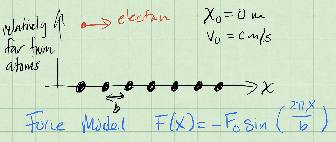
Fig. 21 Lattice chain force model, \(F(x) = -F_0 \sin(\frac{2 \pi x}{b})\)#
Error
Redraw as vector graphic and post SVG
Here the location of the particle and it’s initial velocity are zero. The force model for a chain of atoms in this arrangement is:
where \(b\) is the spacing between the atoms and \(F_0\) is a constant.
We can again find the kinetic energy change and work done by the force:
Using the Work-Energy Theorem, we can write:
Thus, we can find the speed of the object at a given position:
But more importantly, we can derive a potential energy function for the lattice chain. We can write:
where \(C\) is a constant. We can choose \(C\) so that \(U(0) = 0\); only the difference in potential energy matter. Then we have:
This is just another conservative force.
Conservative Forces#
These forces occur frequently enough in physics and their properties are so important that they deserve their own attention. There are a few key properties of conservative forces that we should note:
if the work is independent of the path taken, then the force is conservative.
if the work done by the force is zero for a closed path, then the force is conservative.
if the curl of the force is zero, then the force is conservative.
It turns out that all of these statements are equivalent. And if any one of them is true, the rest hold, and we can develop a potential energy function for the force.
Why do these imply each other?#
Let’s start with the curl of the force. The curl of a vector field is a measure of the rotation of the field. It is a vector differential operator. Operationally, taking the curl amounts to a cross product of the del operator with the vector field. The curl of a vector field \(\vec{F}\) is defined as:
In the event that the curl vanishes, we know that each term in the curl is zero. In this case, we can investigate what this implies about other aspects of the force. We write Stokes’ theorem for the force as:
The left hand side is the integral of the curl of the force over some surface \(S\) with boundary \(C\). The right hand side is the line integral of the force around the boundary of the surface. This theorem holds for any vector field with continuous first derivatives, so most of what we do.
Stokes’s theorem tells us that for any choice of surface \(S\) with boundary \(C\), the line integral of the force around the boundary is equal to the integral of the curl of the force over the surface. If the curl vanishes, then the integral of the curl is zero. Thus, the line integral of the force around the boundary is zero.
This is true for any closed path \(C\). This is the second statement above.
We can equivalent write the integral of the force around a closed path as the work around a different path. The figure below shows these paths \(C_1\) and \(C_2\) that make up the first loop, and the paths \(C_3\) and \(C_4\) that make up the second loop. The work done by the force along each path is shown in the figure.
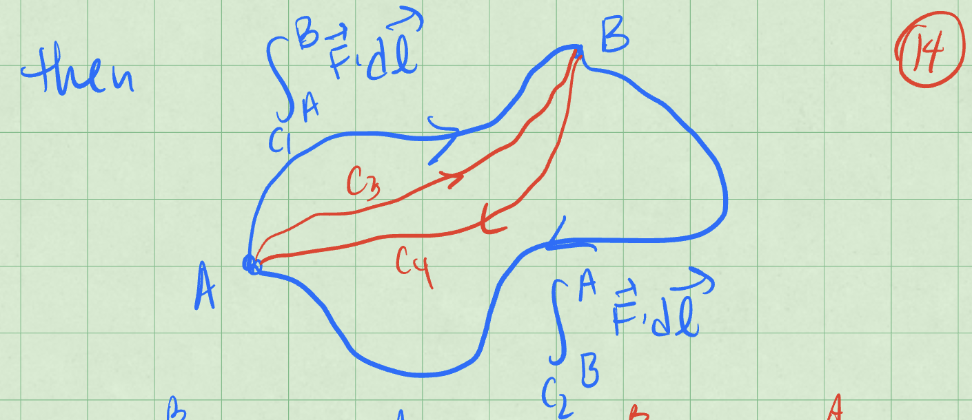
Fig. 22 Illustration of path independence of work for a conservative force.#
Error
Redraw as vector graphic and post SVG
We can take the integral of both paths and write:
Because both paths are closed and start and return to the same point, we can know that each contribution on each part of the path is equal and opposite. Thus, we can write:
This holds for any \(n\) and \(m\) where they make a closed path \(C\). This is the first statement above.
Summary of Results#
We covered a lot fo ground. Let’s remind ourselves of the key results.
The total energy of a system is the sum of the kinetic and potential energies:
We use both \(T\) and \(K\) to represent kinetic energy, and both \(U\) and \(V\) to represent potential energy.
The conservation of energy is:
When all the forces are conservative, energy is conserved. Of course, we are limiting here to mechanical energy.
Conservative forces are those where the work done by the force is independent of the path taken. They have several key properties:
The forces are functions of position only \(\vec{F}(\vec{r})\).
Their curl is zero: \(\nabla \times \vec{F} = 0\).
We calculate the curl as:
The force is given by the negative gradient of the potential energy: \(\vec{F} = -\nabla U\). This stems from the definition of the potential energy as the work done by the force.
We can calculate the gradient as:
The work done by a conservative force is path independent. We can write the work done by a conservative force as:
Linear and Angular Momentum#
We’ve talked about the central conservation laws of classical mechanics:
Conservation of energy - in a process, if energy is conserved, the total energy of the system is the same before and after the process. More strongly, in a closed system, the total energy is constant for any process (\(dE_{sys}/dt=0\)).
Conservation of linear momentum - in a process, if momentum is conserved, the total momentum of the system is the same before and after the process. More strongly, in a closed system, the total vector momentum is constant for any process (\(d\vec{p}_{sys}/dt=0\)).
Conservation of angular momentum - in a process, if angular momentum is conserved, the total angular momentum of the system is the same before and after the process. More strongly, in a closed system, the total vector angular momentum is constant for any process (\(d\vec{L}_{sys}/dt=0\)).
We’ve worked with the conservation of energy a lot because it’s a fundamental concept in physics and it lends itself to a scalar equation analysis. This can be quite a bit simpler in many cases, but an energy only view of the world can be limiting.
Linear Momentum#
As we move into the formal study of linear momentum, we will start with a reminder of the definition of momentum, and the mathematical form of the conservation of momentum.
Linear momentum is a vector quantity defined as the product of an object’s mass and its velocity. It is denoted by the symbol \(\vec{p}\) and is defined as:
where \(m\) is the mass of the object and \(\vec{v}\) is the velocity of the object. The SI unit of momentum is kg m/s. As we later came to understand with Einstein’s special theory of relativity, this definition of momentum is the classical limit of the relativistic momentum:
where \(\gamma\) is the Lorentz factor,
As you can calculate, the relativistic momentum reduces to the classical momentum when the velocity is much less than the speed of light. As \(v/c \rightarrow 0\), \(\gamma \rightarrow 1\), and the relativistic momentum reduces to the classical momentum.
Linear Momentum and Newton’s Second Law#
You have seen in our discussion of Newton’s Second Law that the net force on a system is equal to the mass of the system times the acceleration of the system. This can be written as:
However, this definition and our thinking here with it is a bit limited. What about systems of objects that are interacting with each other? What about deformable systems? What happens if something is shedding mass, like a rocket or jet?
Newton’s definition from the Principia is a bit more general. He defines the force in terms of the rate of change of the body’s momentum:
We can extend that definition to a system of objects, where the net force on the system is equal to the rate of change of the total momentum of the system:
The second step might not be obvious, but by working through a few examples we can see how this is a more useful and general definition of force.
Forces internal to a system zero out#
Consider an abstract system of \(N\) particles. You might think of them as point particles but they could be extended objects. They experience outside forces and internal forces; i.e., we go a tag all the particles in our system and we can tell which ones are interacting with each other. We can also tell which ones are interacting with the outside world. This is a bit silly, but it can help us visualize what we are arguing below.
The total force on the system is given by the sum of all the masses times the acceleration of each particle:
where the last term is the net force on the \(ith\) particle. For a given object, \(i\), the net force is the sum of all the forces acting on it, both internal and external,
Here these internal forces are pairwise interactions between the particle \(i\) and every other particle in the system,
where the sum is over all particles that are not \(i\) because there’s no force between a particle and itself.
Cool, what happens to the internal force equation when we sum over all particles in the system?
Concrete Examples#
We have a generic setup, let’s see what happens when we apply this to a few examples: 2 particles, 3 particles, and then N particles.
Two Particles#
With two particles the sum is easy to write out fully.
By Newton’s Third Law, the force of particle 1 on particle 2 is equal and opposite to the force of particle 2 on particle 1. The internal forces cancel out and the net force on the system is the sum of the external forces.
So here the internal forces sum to zero.
Three Particles#
We can write this out in a similar way.
We can group these terms by Newton’s Third Law pairs.
Every interaction on body \(i\) has a corresponding equal and opposite interaction on body \(j\), and the internal forces are again zero.
N Particles#
Clearly, there seems to be a pattern here. Namely that the internal forces are always zero. We can write out the sum for \(N\) particles in a way that suggests this is always true.
And where we make a switch in the sum terms, so we can counting the force from each interaction in each term in the sum to make it clear why the internal forces sum to zero.
Internal forces will always appear as third law pairs, so the internal interactions will always sum to zero. This is a very powerful result.
For a given system, only external forces can change the momentum.
Mathematical Form of Conservation of Linear Momentum#
Let’s look back at the system momentum,
If we take the time derivative of the system momentum, and assume we have point particles, so the masses are not changing,
The net force on the system is given by,
Should there be no external forces, then,
And thus there is no change momentum of the system,
So if the system has no external forces, the total momentum of the system is conserved. We can propose a discrete extension to this form above where
And thus, it’s easy to see:
If there are external forces, then we also have a prediction equation for how the energy will change in a small time step \(\Delta t\):
so that,
Angular Momentum#
Angular momentum is a complex and rich quantity that has deep connections to the shape and structure of a system. The “configuration” or how it is distributed in space can have a big impact on the dynamics of a system. Our study of classical angular momentum will be a stepping stone to our study of quantum angular momentum and the spin of particles.
Quantum Mechanical Spin
Spin is a quantum mechanical property that is not related to the rotation of a particle, but it is a form of angular momentum, and it’s essential to the structure of the universe - it tells us if we have fermionic or bosonic particles, it is what gives us the Pauli Exclusion Principle, and it is what gives us the Zeeman Effect and the Stark Effect.
For the moment, we will limit ourselves to classical angular momentum and we will focus on the abstract case of a single particle. As we work through the semester, we will revisit angular momentum and introduce how to work with distributions of mass and extended objects.
Definition of Angular Momentum#
For a particle with a momentum \(\vec{p}\), the angular momentum is defined as the cross product of the position vector \(\vec{r}\) and the momentum vector \(\vec{p}\),
This is a quantity that depends on the location of the particle relative origin of coordinates. This means you have some latitude in choosing the origin of coordinates, and you can choose the origin to simplify the problem.
This also means the angular momentum is a vector quantity, and it points in the direction perpendicular to the plane defined by the position and momentum vectors.
When is Angular Momentum Conserved?#
We can ask this by computing the time derivative of the angular momentum,
We did a calculation like this on a homework where we computed
Let’s apply it here:
If we assume that \(\dot{m}=0\), then we can write the time derivative of the momentum as,
We group the terms in the time derivative of the angular momentum,
The first term the cross product of the velocity with itself \(\vec{v}\times\vec{v}\), and is zero, and the second term is the cross product of the position vector with the acceleration,
So the time derivative of the angular momentum is the net torque on the system!
If the net torque on the system is zero, then the angular momentum is conserved, and it is a constant of the motion.
If there’s a net torque, we have a discrete update equation for the angular momentum,
Are we sure there are no internal torques that matter?#
We can ask the same question we asked about internal forces. Are there internal torques that matter? As before, let us define the total force on particle \(i\) as the sum of internal and external forces,
We assume there are no external forces, and so the net force on the system is the sum of the internal forces,
For given object, we observe an angular momentum \(\vec{l}_i\) that is the cross product of the position vector and the momentum vector. So the time derivative of the \(i\)th particle’s angular momentum is,
If the total angular momentum of the system is the sum of the angular momenta of the particles,
then the time derivative of the total angular momentum is,
Recall that \(\vec{F}_i = \sum_{j\neq i}^{N} \vec{F}_{ij}\). So we can rewrite the time derivative of the total angular momentum as,
But note that \(\vec{r}_i \times \vec{F}_{ij} = -\vec{r}_j \times \vec{F}_{ji}\), so the resulting expression gives us,
So if the internal forces are parallel to the separation between the particles, then the internal torques sum to zero, and the total angular momentum of the system is conserved. So things like the gravitational force, the electric force, and spring forces are all internal forces that do not contribute to the net torque on the system.
And thus,
Understand the conditions under which the total momentum of a system is conserved.
Derive and apply the discrete update equation for momentum in the presence of external forces.
Define angular momentum for a single particle and understand its dependence on the choice of the origin.
Explore the relationship between angular momentum and torque, and derive the conditions for angular momentum conservation.
Analyze the role of internal forces and torques in the conservation of angular momentum.
Understand how forces like gravity, electric forces, and spring forces contribute to the net torque on a system.
Practice deriving time derivatives of angular momentum and interpreting their physical significance.
Use vector calculus to analyze the dynamics of systems with multiple particles.
Understand the principle of energy conservation and its application to physical systems.
Derive and apply equations for energy changes in systems with external forces.
Analyze the interplay between kinetic, potential, and total energy in dynamic systems.