Homework 13 (Due December 6th)
Homework 13 finishes our discussion of magnetism by focusing on the vector potential, which is a useful tool for calcualting the magnetic field in some problems, and magnetic dipoles. It also introduces the idea of magnetic fields in matter using the H-field.
1. Vector Potential I
- A long (infinite) wire (cylindrical conductor, radius $R$, whose axis coincides with the $z$ axis) carries a uniformly distributed current $I_0$ in the $+z$ direction. Assuming $\nabla \cdot \mathbf{A} = 0$ (the “Coulomb gauge”), and choosing $\mathbf{A}=0$ at the edge of the wire, show that the vector potential inside the wire could be given by $A= c I_0(1-s^2/R^2)$. Find the constant $c$ (including units.) Things to explicitly find/discuss: What is the vector direction of $\mathbf{A}$? (Does it “make sense” in any way to you?) Is your answer unique, or is there any remaining “ambiguity” in $\mathbf{A}$? (Note that we’re not asking you to derive $\mathbf{A}$ from scratch, just to see that this choice of A “works”)
- What is the vector potential outside that wire? (Make sure that it still satisfies $\nabla \cdot \mathbf{A} = 0$, and make sure that $\mathbf{A}$ is continuous at the edge of the wire, consistent with part 1). Here again, is your answer unique, or is there any remaining “ambiguity” in $\mathbf{A}(outside)$?
2. Vector Potential II
Griffiths Fig 5.48 is a handy “triangle” summarizing the mathematical connections between $\mathbf{J}$, $\mathbf{A}$, and $\mathbf{B}$ (like Fig. 2.35) But there’s a missing link, he has nothing for the left arrow from $\mathbf{B}$ to $\mathbf{A}$. Note the equations defining $\mathbf{A}$ are very analogous to the basic Maxwell’s equations for $\mathbf{B}$:
\[\nabla \cdot \mathbf{B} = 0 \leftrightarrow \nabla \cdot \mathbf{A} = 0\] \[\nabla \times \mathbf{B} = \mu_0\mathbf{J} \leftrightarrow \nabla \times \mathbf{A} = \mathbf{B}\]-
So $\mathbf{A}$ depends on $\mathbf{B}$ in the same way (mathematically) the $\mathbf{B}$ depends on $\mathbf{J}$. (Think, Biot-Savart!) Use this idea to just write down a formula for $\mathbf{A}$ in terms of $\mathbf{B}$ to finish off that triangle.
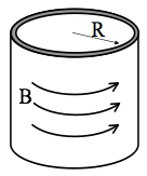
- In lecture notes (and/or Griffiths Ex. 5.9) we found the $\mathbf{B}$ field everywhere inside (and outside) an infinite solenoid (which you can think of as a cylinder with uniform surface current flowing azimuthally around it (see figure below). See Griff. Fig 5.35. Use the basic idea from the previous part of this question to, therefore, quickly and easily just write down the vector potential $\mathbf{A}$ in a situation where $\mathbf{B}$ looks analogous to that, i.e. $\mathbf{B} = C\delta(s-R)\hat{\phi}$, with $C$ constant. Also, sketch this $\mathbf{A}$ for us, please. (You should be able to just “see” the answer, no nasty integral needed!)
- For you to discuss: What physical situation creates such a $\mathbf{B}$ field? (This is tricky - think about it!) Also, if I gave you some $\mathbf{B}$ field and asked for $\mathbf{A}$, can you now think of an “analogue method”, i.e. an experiment where you could let nature do this for you, instead of computing it? It’s cool - think about what’s going on here. You have a previously solved problem, where a given $\mathbf{J}$ led us to some $\mathbf{B}$. Now we immediately know what the vector potential is in a very different physical situation, one where $\mathbf{B}$ happens to look like $\mathbf{J}$ did in that previous problem.
3. Coordinate Free Dipole Equation
In class we derived the magnetic field formula for the magnetic moment of a pure dipole which points in the z direction, located at the origin:
\[\mathbf{B} = \dfrac{\mu_0 m}{4 \pi r^3}(2 \cos \theta\,\hat{r} + \sin \theta\,\hat{\theta})\]Here $\mathbf{m}=I\mathbf{a}$ ($\mathbf{a}$ is the area vector of our tiny dipole) But sometimes $\mathbf{m}$ points in another direction than just $z$-hat! A more elegant way to write B which does not explicitly depend on any choice of coordinate axes is:
\[\mathbf{B} = \dfrac{\mu_0}{4 \pi r^3}(3 (\mathbf{m}\cdot\hat{r})\hat{r} - \mathbf{m})\]- For this problem, assume the second equation above is correct, define your $z$-axis to lie along the direction of the magnetic moment $\mathbf{m}$, and show that this leads back to first equation.
Coordinate free formulas are nice, because now you can find B for more general situations!
4. Semi-classical electron dipole moment
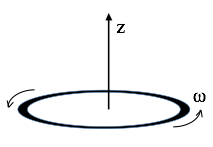
A thin uniform solid torus (a “donut”) has total charge $Q$, mass $M$, radius $R$. It rotates around its own central axis at angular frequency $\omega$, as shown.
- Find the magnetic dipole moment $m$ of this rotating donut. What are the SI units of dipole moment?
- Compute the ratio $m/L$, the “magnetic dipole moment” divided by the angular momentum. This is called the “gyromagnetic ratio”.
- What is the gyromagnetic ratio for a uniform spinning sphere? HINT: This question really doesn’t require any additional calculating: picture the sphere as a bunch of rings, and apply the result of part 2.
- In quantum mechanics, the angular momentum of a spinning electron is $\hbar/2$. Use your results above to deduce the electron’s magnetic dipole moment (in SI units.)
Note: This “semi-classical” calculation is low by a factor of almost exactly 2. Dirac developed a relativistic form of quantum mechanics which got the factor of 2 right in the 1930’s. In the ‘40’s, Feynman, Schwinger, and Tomonaga calculated tiny extra corrections arising from QED (Quantum electrodynamics) For fun, find the current best-value for the electron magnetic dipole moment. If you compare theory and measurement, you will be extremely impressed at the agreement (~12 digits!) It may make you “believe” in quantum physics in a way you might not have before! That’s not how it works in practice though- people use this measurement to extract a fundamental constant of nature, and then use that value to predict OTHER experiments.
5. Bound Currents I
Consider a long magnetic rod, radius $a$. Imagine that we have set up a permanent magnetization $\mathbf{M}(s,\phi,z) = c \hat{z}$, with $c$ = constant. Neglect end effects, assume the cylinder is infinitely long.
- Calculate the bound currents $\mathbf{K}_b$ and $\mathbf{J}_b$ (on the surface, and interior of the rod respectively).
- What are the units of $c$?
- Use these bound currents to find the magnetic field inside and outside the cylinder. (Direction and magnitude)
- Find the $\mathbf{H}$ field inside and outside the cylinder, and verify that $\oint \mathbf{H} \cdot d\mathbf{l} = I_{free}$ works. Explain briefly in words why your answer might be what it is.
- Now relax the assumption that it is infinite - if this cylinder was finite in length ($L$), what changes? Sketch the magnetic field (inside and out). Briefly but clearly explain your reasoning. Please draw two such sketches, one for the case that the length $L$ is a few times bigger than a (long-ish rod, like a magnet you might play with from a toy set), and another for the case $L \ll a$, which is more like a magnetic disk than a rod.
6. Bound Currents II
Like the last question, consider a long magnetic rod, radius $a$. This time imagine that we can set up a permanent azimuthal magnetization $\mathbf{M}(s,\phi,z) = c s \hat{\phi}$, with $c$ = constant, and $s$ is the usual cylindrical radial coordinate. Neglect end effects, assume the cylinder is infinitely long.
- Calculate the bound currents $\mathbf{K}_b$ and $\mathbf{J}_b$ (on the surface, and interior of the rod respectively).
- What are the units of $c$?
- Use these bound currents to find the magnetic field $\mathbf{B}$, and also the $\mathbf{H}$ field, inside and outside. (Direction and magnitude)
7. Bound Currents III
Once more, consider a very long cylinder (radius $R$) with a permanent magnetization, this time again parallel to the axis: $\mathbf{M} = c s \hat{z}$, (where $c$ is a constant, and $s$ is the usual distance from the cylinder’s axis). There is no free current anywhere.
- Find the magnetic field inside and outside the cylinder by figuring out the bound current everywhere and then figure out $\mathbf{B}$ created by those.
- Let’s find the $\mathbf{B}$ field inside and outside another way! This time, use Ampere’s law in the form: $\oint \mathbf{H} \cdot d\mathbf{l} = I_{free}$, and then use the standard relation, $\mathbf{H} = \frac{1}{\mu_0}\mathbf{B} - \mathbf{M}$, to get $\mathbf{B}$. (It should agree with part 1)