Day 22 - Damped Oscillations

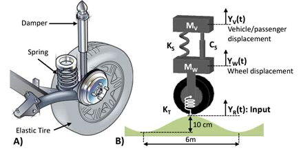
Shock absorbers are a type of damped oscillator.

They must be tuned to the weight of the car and the type of driving.

---

Announcements

• Homework 5 is due on today (late on Sunday)

  • Anyone may request an extension for HW5 up to one week, no questions asked. Just email me.

• Homework 6 is due the following Friday (late on Sunday)

  • Again, anyone may request an extension for HW6 up to one week, no questions asked. Just email me.

• Class next Monday, maybe?

---

Reminders

We are solving the harmonic oscillator equation: $\(\ddot{x} + \omega_0^2 x = 0\)$

We have general solutions of the form:

\[x(t) = A\cos(\omega_0 t + \delta)\]

\[x(t) = A\sin(\omega_0 t + \delta)\]

\[x(t) = A\cos(\omega_0 t) + B\sin(\omega_0 t)\]

We seek complex solutions of the form:

\[x(t) = Ae^{(i\omega_0 t + \delta)}\]

---

Reminders

We denote a complex number in “Cartesian form” as:

\[z = x + iy\]

Here, \(x\) is the real part and \(y\) is the imaginary part; both are real numbers.

\[Re(z) = x \qquad Im(z) = y\]

The complex conjugate of \(z\) is:

\[z^* = \bar{z} = x - iy\]

---

Reminders

We can also write a complex number in “polar form” as:

\[z = Ae^{i\delta}\]

where \(A\) is the magnitude of the complex number and \(\delta\) is the phase. Both are real numbers.

\[A = |z| = \sqrt{x^2 + y^2} \qquad \delta = \tan^{-1}\left(\frac{y}{x}\right)\]

The complex conjugate of \(z\) is: $\(z^* = \bar{z} = Ae^{-i\delta}\)$

---

Reminders

The product of a complex number and its complex conjugate is:

\[z\bar{z} = (x + iy)(x - iy) = x^2 + y^2 = A^2\]

The sum of a complex number and its complex conjugate is:

\[z + \bar{z} = (x + iy) + (x - iy) = 2x = 2Re(z)\]

The difference of a complex number and its complex conjugate is:

\[z - \bar{z} = (x + iy) - (x - iy) = 2iy = 2iIm(z)\]

---

Clicker Question 22-1

A complex number \(z\) is plotted in the complex plane such that \(z\) lies in the second quadrant.

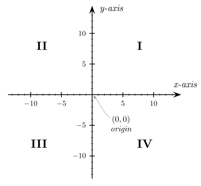
Where does the complex conjugate \(z^*\) lie?

1. In the first quadrant.

2. In the second quadrant.

3. In the third quadrant.

4. In the fourth quadrant.

---

Visualizing the Complex Solution

We constructed a solution of the form:

\[Ae^{i(\omega t-\delta)}\]

We can plot it in the complex plane and see the real and imaginary parts, and how they change in time.

---

Visualizing the Complex Solution

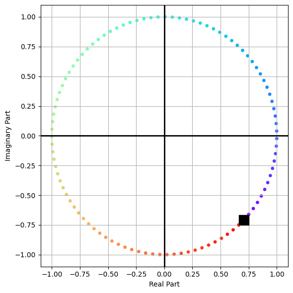
We can plot the solution on the complex plane. For this, \(\delta = \pi/4\), and the amplitude is \(A=1\).

The solution rotates counterclockwise in the complex plane, following the rainbow from violet to red.

---

Projecting the Real Solution

The real part is just the projection of the complex solution onto the real axis. Just how far along the real axis is the solution at any given time.

That looks like a time trace, but not quite, it’s the real projection. The colors scheme is the same as before.

---

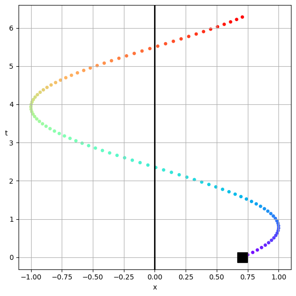
The Time Trace of the Solution

We just flip the axes to produce the time trace that you are used to seeing. The color scheme is the same as before.

---

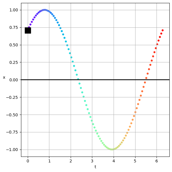
Table Activity 22-2

We constructed a solution for the weakly damped harmonic oscillator:

\[x(t) = e^{-\beta t} \left(C_1e^{i\omega_1 t} + C_2e^{-i\omega_1 t}\right)\]

where \(\omega_1 = \sqrt{\omega_0^2 - \beta^2}\).

• What is the physical meaning of \(\beta\)?

• Sketch this solution, you can choose parameters, or just roughly sketch it.

• What happens to the amplitude of the solution as time goes on?

• Can you describe the mathematical “envelope” of the solution?

• What is the physical meaning of this envelope?

Click when you and your table are done.

---

Exercise 3

The apparatus below is a massless wheel of radius \(R\) that is mounted to a frictionless axle. A small, dense piece of clay with mass \(M\) is glued to edge of the wheel as shown. Another mass \(m\) hangs from a massless string that is wrapped around the wheel. We can assume the string is inextensible and does not slip, and the system is in a uniform gravitational field.

---

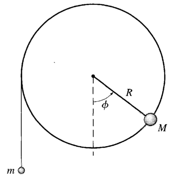
Exercise 3

We can show that this complicated system is still one-dimensional (at least in space) and then we can see the effects of parameters like \(m/M\).

• In terms of the rotation angle \(\phi\) of the wheel, write down the total potential energy \(U(\phi)\) of the system of both masses. Take note of any constraints that you use to write this as a 1D problem. When working this kind of problem, every object-Earth pair has gravitational potential energy and we must have the same zero of potential energy for every pair.

---

Exercise 3

• Use this potential energy to find values of \(m\) and \(M\) for which there are “fixed points”, “critical points”, or what we sometimes call “equilibrium points”. The language we use comes from different fields, but the concept is the same. What is the condition for the existence of any critical points?

• Describe the fixed points, determine their stability, and explain why they make sense in terms of the expected motion.

---

Exercise 3

• Plot the potential energy for two different values of \(m/M\) and explain the differences in the potential energy graphs. Consider cases when you observe very different motion. Think about an initial condition where the mass \(m\) is at rest and the wheel is at rest. What happens when you release the mass \(m\) for your two cases?

• Determine the value of \(m/M\) for which the system begins to exhibit oscillations (if released from \(\phi=0\)).