Week 4 - Why does fluid drag complicate things?#
As an object moves through the fluid, the molecules of the fluid collide with the object and exert a force on it. This collision changes the momentum oof the object just a little bit. The collision does so in a random way, but the average effect of all those collisions is to exert a force on the object that is proportional to a function of the object’s velocity, \(F(v)\). In some cases those collisions occur such that they make an impact; other times they might approach the object more slowly and slide over it in a more frictional interaction. These two behaviors are both fluid drag, but they are different forms.
The first form (\(F \sim v^2\)) describes the behavior of things like a skydiver falling, a high-speed car, or a baseball thrown through the air. But it can also be valid for the movement of fish in water, or a submarine moving through the ocean. Through those collisions, the distribution of those forces can cause intra-body forces, which can result in damage or deformation of the object. However, we often model the body as solid and focus on the way this form of air resistance changes the motion.
This form of air resistance cannot describe the behavior of objects approaching the speed of sound in the fluid. Objects moving a speeds that high can produce shock fronts that forces the fluid to go through abrupt changes in density, pressure, and temperature. Below is a figure of a shock front produced the nose of a jet flying at supersonic speeds.

The second form (\(F \sim v\)) describes the flow of a viscous fluid around a solid object. You might think of this as pulling an object through some viscous oil, honey, or even molasses. The movement of the fluid around the object exerts a force and slows the motion of the object. In water, this form can explain the motion of some of the smallest creatures on Earth, like the water bear, an amoeba, or a paramecium.
What is interesting here is that these creatures have had to adapt to this form of fluid drag. Edward Purcell wrote a paper in 1977 called Life at Low Reynolds Number that describes the motion of these creatures. He demonstrates that the physics in this regime requires creature to have adapted forms of locomotion that can take advantage of that environment.
Why do we often neglect air resistance?#
We’re in the business of making models of physical systems using the concepts and tools of Classical Mechanics. We’ve focused on Newton’s Laws, which are a formulation of mechanics that starts from the concept of the force.
We often start with that approach because the mathematical tools that we have available to us when we are first learning physics are geometry and algebra. Forces are a vector concept and Newton’s Second Law is a vector equation that holds in each of the three dimensions of space. This formulation lends itself to a decomposing problems often into two or three separate problems, one for each dimension, and then using some algebra to solve the problems. However, that mathematics limits the kinds of explorations we can do.
This is one reason why we neglect air resistance in our first explorations of motion. Our models of air resistance are more complicated and require more advanced mathematics to solve. The equations of motion can be coupled and non-linear. In some cases, we cannot solve the equations of motion analytically and must resort to numerical methods like Euler’s method, or the more often used Runge-Kutta method.
The Reynolds Number#
The different forms of fluid drag are often described by a dimensionless number called the Reynolds Number. The Reynolds number is a ratio of the inertial forces to the viscous forces in a fluid.
What are inertial forces? They are the ones associated with resistance to motion, the mass of the object. The more massive the object in a given setup, the higher the inertial contribution.
What are viscous forces? They are the ones associated with the interaction of the fluid with the object. The more viscous the fluid - the harder it for is to flow under the same conditions, the higher the viscous contribution.
The Reynolds number is defined as:
where \(\rho\) is the density of the fluid, \(v\) is the velocity of the object in that fluid, \(L\) is a characteristic length of the object, and \(\mu\) is the dynamic viscosity of the fluid.
You can probably see who the Reynolds number characterizes the system of the object and the fluid as their are properties of both the object and the fluid in the equation. The Reynolds number can be measured quite accurately in a lab because the laboratory setups are typically designed to make the measurement of the Reynolds number easier. We will often estimate it in theoretical physics.
What is a characteristic length?#
This length is a generic length scale associated with the flow, this can be the order of magnitude size of the object, or, in the absence of an object, the same for the pipe or channel in which the flow is occurring. If it’s an airplane, it can be the wingspan, or the length of the fuselage. If it’s a car, it can be the length of the car. If it’s a sphere, it can be the radius, and so on.
What is dynamic viscosity?#
Viscosity is the measure of the fluid’s resistance to flow. It’s how the fluid slides past itself. It’s a bit of a harder quantity to describe, but you can think of it as the “stickiness” of the fluid. The higher the viscosity, the more sticky the fluid is – really, for a given setup, the more viscous fluid will flow more slowly. The lower the viscosity, the higher tendency for a fluid to flow. Compare honey to water in the same vessel and temperature, and you’ll observe the difference in viscosity.
Measuring viscosity#
We can sometimes measure viscosity with a viscometer, which uses a capillary tube to measure the time it takes for a fluid to flow through a tube of known dimensions. However, this works best for Newtonian fluids, which are fluids that have a constant viscosity.
Non-Newtonian fluids (in your kitchen)#
Not all fluids are Newtonian, and some fluids have a viscosity that changes with the rate of flow. These non-Newtonian fluids can be shear thinning or shear thickening. Shear thinning fluids become less viscous when they are stirred or shaken, while shear thickening fluids become more viscous when they are stirred or shaken.
Below is a video from America’s Test Kitchen that demonstrates the behavior of a non-Newtonian fluid. The fluid is made from cornstarch and water, and it’s called oobleck.

Source: https://www.youtube.com/watch?v=FrLh1GILomc
The physics of cooking is fascinating and covers the field of soft matter physics. There’s a free course on the subject offered by Harvard and EdX.
Low Reynolds Number Flows#
A low Reynolds number flow is a flow where the viscous forces dominate the inertial forces. The object is moving slowly, or the fluid is very viscous, or the object is very small. We typically think of these flows as being in the range of \(Re < 1\). In these flows, the motion of the fluid is typically laminar; it flows in fairly smooth and parallel layers. Low Reynolds number flows can produce dynamics that is counterintutive. Below are a couple videos that explain the physics of low Reynolds number flows.
Physics of Life - Life at Low Reynolds Number (15 minute video)#
This video focuses on the biological aspects of the problem as the physics of low Reynolds numbers is important for understanding the motion of microorganisms.

G.I. Taylor’s Low Reynolds Number Flows (32 minute video)#
This video is a classic from G.I. Taylor who was a physicist interested in sharing the conceptual beauty of physics with the general public. He was also a pioneer in the field of fluid mechanics. In fact, Taylor’s groundbreaking paper on the stability of fluid flows between two rotating cylinders set off studies into turbulence. The Taylor-Couette flow is a critical tool for studies of turbulence.

High Reynolds Number Flows#
In high Reynolds number flows, the inertial forces dominate the viscous forces. The object is moving quickly, or the fluid is not very viscous, or the object is very large. We typically think of these flows as being in the range of \(Re > 1000\). In these flows, the motion of the fluid is typically turbulent. Turbulent flows are characterized by chaotic and irregular motion. The fluid moves in a complex and unpredictable way, with eddies and vortices forming and dissipating. Turbulent flows can be very difficult to predict and model, but they are also very common in nature.
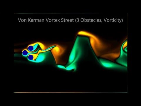
Von Kármán’s Vortex Street (2 minute video)#
The von Kármán vortex street is a pattern of alternating vortices that can form when a fluid flows past a “bluff” body, such as a cylinder or a sphere. The vortices are shed from the body in a regular pattern, creating a repeating pattern of alternating vortices. The von Kármán vortex street is an example of a high Reynolds number flow, and it can be used to study the behavior of turbulent flows. Below is a video of a von Kármán vortex street simulation.
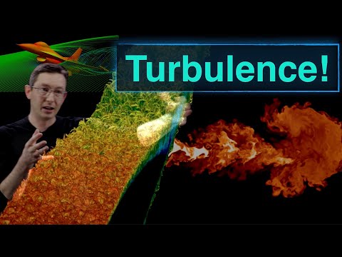
Turbulent Flow (24 minute video)#
Turbulence is a major research area in science. We don’t fully understand it. We are trying to determine what triggers it, how to control it, and how to predict if and when it will occur. The problem of turbulence is frequently multi-scale such that behavior at one time or length scale is not well explained or connected to another scale. Additionally, the mathematics of turbulence is very difficult. It makes for an interesting and challenging research area. Below is a video that explains the some of the physics of turbulence. The first 4 minutes or so are at least worth watching.