Week 6 - Notes: Stability and Energy

You have likely already heard of the concept of stability in other classes or contexts. The idea that something is “stable” is a well understood concept in everyday language, but here we mean to put some precision on the statement.

• What do we mean by stable?

• And what forms of stability are there?

• What are the implications of stability for the behavior of a system?

We will start this from the perspective of force and then relate it to the potential energy. Ultimately, we will develop a toolkit for understanding the stability of a system and how to analyze it.

Further, we will introduce the idea of fixed points and how they relate to stability. These fixed points, or equilibrium points, are the points where the system is at rest, or it would be if it were not disturbed. They are important to identify because they are the first concept in the larger narrative of stability. Later, we will see how systems can produce other structures like limit cycles and chaotic attractors. Indeed, in some cases, we can parameterize the system, by choosing a tuneable variable, to produce any of these structures.

What is an equilibrium point?

This might have an obvious answer to you if you think about a vertical pendulum. Obviously, the bottom of the swing has some special meaning, and it is the point that the pendulum will return to if it is not disturbed. As, surely, you can surmise, this is an equilibrium point for this system.

But what about the location at the top of the swing? The location directly opposite the bottom of the swing? It turns out that is also an equilibrium point. But there is something very different about these two points.

The bottom of the swing is a stable equilibrium point, while the top of the swing is an unstable equilibrium point. This basic idea that we can identify points in the system where the system is at rest is a powerful concept. Moreover, we already have some intuition about the stability of these points; for example, the bottom of the swing is a lower potential energy state, while the top of the swing is a higher potential energy state.

How can we identify equilibrium points?

Starting from Newton’s second law, we can write the equation of motion for a system. This equation will be a differential equation that describes how the system evolves in time. For the pendulum without a small angle approximation, we have the following equation of motion:

\[m L \ddot{\theta} = -m g \sin(\theta)\]

Where \(m\) is the mass of the pendulum, \(L\) is the length of the pendulum, \(g\) is the acceleration due to gravity, and \(\theta\) is the angle of the pendulum from the vertical; measured from the bottom of the swing.

To find the equilibrium points we search for the points where \(\ddot{\theta} = 0\). This is the point where the system is at rest, or instantaneously at rest. In this case, we have:

\[0 = -g \sin(\theta),\]

\[\sin(\theta) = 0.\]

Now, we know that the angle theta here is measurable around the entire circles as we did not make the small angle approximation. Thus, we find that the equilibrium points are at:

\[\theta = 0\;\mathrm{and}\;\theta = \pi,\]

corresponding to the bottom and top of the swing, respectively. There are in fact an infinite number of equilibrium points for this system, but these are the only unique points. The others would correspond to multiple rotations around the circle.

What is happening here? Where does energy come into play?

What we’ve done is use the equation of motion to find the points where the system is at rest. But we can also think of this in terms of the potential energy of the system. The strength of the potential energy view is that there’s another representation of the system that can be used to understand the stability of the equilibrium points, namely the graph of the potential energy. We can use this energy landscape to help us see the stability of the equilibrium points.

The potential energy of the pendulum that we have been discussing is given by:

\[U(\theta) = -m g L \cos(\theta).\]

Let’s graph this potential energy and see what it looks like.

import numpy as np
import matplotlib.pyplot as plt
%matplotlib inline

plt.style.use('seaborn-v0_8-colorblind')

theta = np.linspace(-np.pi, np.pi, 1000)
U = -9.8 * np.cos(theta)


fig = plt.figure(figsize=(8, 6))

plt.plot(theta, U)

plt.xlabel(r'$\theta$')
plt.ylabel(r'$U(\theta)$')

plt.xticks([-np.pi, -np.pi/2, 0, np.pi/2, np.pi],
           [r'$-\pi$', r'$-\pi/2$', r'$0$', r'$\pi/2$', r'$\pi$'])
plt.yticks([-10, -5, 0, 5, 10], ['-10', '-5',  '0', '5', '10'])

plt.title('Potential Energy of a Pendulum')

plt.grid()
plt.tight_layout()
plt.show()

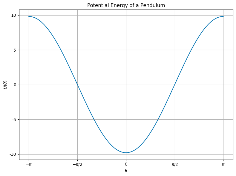
We can see where the equilibrium points are by noticing they are the minima and maxima of the potential energy. In fact, these fixed points are the extrema of the potential energy. The bottom of the swing is a minimum, while the top of the swing is a maximum. This is a general property of fixed/equilibrium points that are derived from a potential energy function.

We also can see then how we might find these points by looking at the potential energy. Given a potential energy function, we can find the equilibrium points by finding the extrema of the potential energy.

Let’s return to the pendulum example.

\[U(\theta) = -m g L \cos(\theta).\]

The first derivative of the potential energy is:

\[\frac{dU}{d\theta} = m g L \sin(\theta).\]

Setting this equal to zero, we find the equilibrium points:

\[\sin(\theta) = 0,\]

\[\theta = 0\;\mathrm{and}\;\theta = \pi.\]

This is the same result we found from the equation of motion. This approach is generally applicable to potential energy functions because the equation of motion is derived from the potential energy through it’s gradient. In 1D,

\[m a = F = -\frac{dU}{dx}.\]

Or in 3D,

\[m \mathbf{a} = \mathbf{F} = -\nabla U.\]

In the case of the pendulum, we have:

\[m L \ddot{\theta} = -\frac{dU}{d\theta},\]

\[m L \ddot{\theta} = -m g L \sin(\theta).\]

How can we determine the stability of an equilibrium point?

Clearly from our intuition, the bottom of the swing is a stable equilibrium point, while the top of the swing is an unstable equilibrium point. But how can we determine this mathematically? We have found that the equilibrium points are at \(\theta = 0\) and \(\theta = \pi\).

Let’s plot the potential energy again and include the equilibrium points. We know which are stable and which are unstable, but let’s see if we can determine this from the potential energy.

import numpy as np
import matplotlib.pyplot as plt
%matplotlib inline

plt.style.use('seaborn-v0_8-colorblind')

theta = np.linspace(-np.pi, np.pi, 1000)
U = -9.8 * np.cos(theta)


fig = plt.figure(figsize=(8, 6))

plt.plot(theta, U)
plt.plot(0, -9.8, 'C2*', label='stable', markersize=20)
plt.plot(-np.pi, 9.8, 'C3*', label='unstable', markersize=20)
plt.plot(+np.pi, 9.8, 'C3*', markersize=20)


plt.xlabel(r'$\theta$')
plt.ylabel(r'$U(\theta)$')

plt.xticks([-np.pi, -np.pi/2, 0, np.pi/2, np.pi],
           [r'$-\pi$', r'$-\pi/2$', r'$0$', r'$\pi/2$', r'$\pi$'])
plt.yticks([-10, -5, 0, 5, 10], ['-10', '-5',  '0', '5', '10'])

plt.title('Potential Energy of a Pendulum')
plt.legend()

plt.grid()
plt.tight_layout()
plt.show()

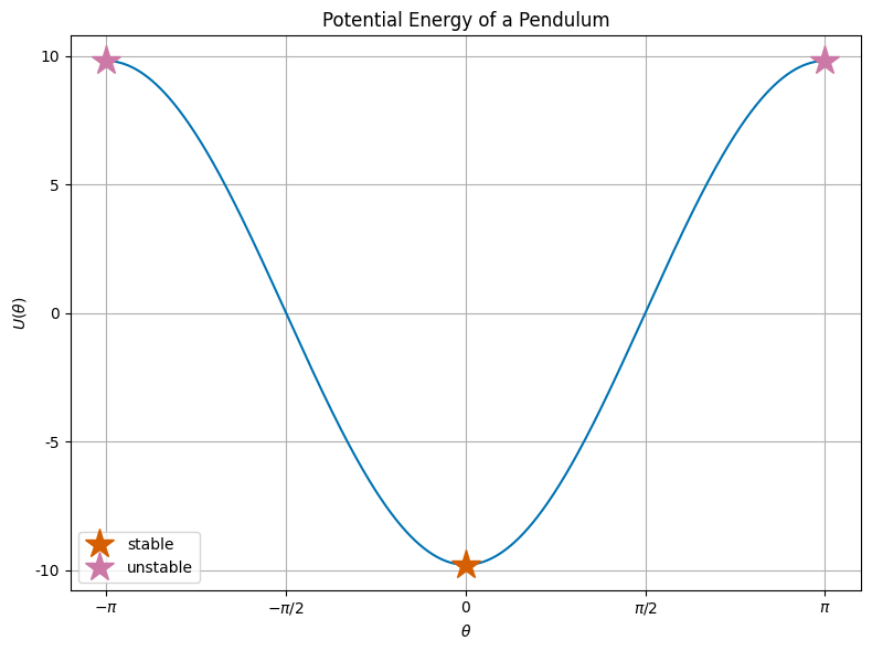
So it’s clear that the equilibrium points are the extrema of the potential energy. We can determine their stability in the same way we identified them. We look at the local curvature of the potential energy at the equilibrium points. If we find that the second derivative of the potential energy is positive, then the equilibrium point is stable. If the second derivative is negative, then the equilibrium point is unstable.

Let’s calculate the second derivative of the potential energy for the pendulum:

\[U(\theta) = -m g L \cos(\theta),\]

\[\frac{dU(\theta)}{d\theta} = m g L \sin(\theta),\]

\[\frac{d^2U(\theta)}{d\theta^2} = m g L \cos(\theta).\]

At the bottom of the swing, \(\theta = 0\), we have:

\[\frac{d^2U(\theta = 0)}{d\theta^2} = m g L > 0.\]

At the top of the swing, \(\theta = \pm\pi\), we have:

\[\frac{d^2U(\theta = \pm\pi)}{d\theta^2} = -m g L < 0.\]

Thus, we have confirmed that the bottom of the swing is a stable equilibrium point, while the top of the swing is an unstable equilibrium point.

Our new toolkit

We now have a set of tools to help us understand the stability of a system. We can find the equilibrium points by setting the acceleration to zero, or by setting the first derivative of the potential energy to zero. We can determine the stability of these points by looking at the curvature of the potential energy at these points.

If we have a system that can be described fully by a potential energy function, we can use this toolkit to understand the stability of the system. We will develop a broader class of tools for when the system is not fully described by a potential energy function, or for multi-dimensional systems. But this is a good start.

1. Write out the potential energy function for the system, \(U(x)\).

2. Find all the extrema, \(x^*\), of the potential energy by setting the first derivative to zero, \(\frac{dU}{dx} = 0\). These are the equilibrium points.

3. Evaluate the second derivative of the potential energy at each of these points, \(\frac{d^2U(x=x^*)}{dx^2}\). If this is positive, the equilibrium point is stable. If it is negative, the equilibrium point is unstable. If it’s zero, it might be metastable.