
Day 10 - Integrating EOMs Numerically#
For Friday, please submit questions.

Announcements#
Homework 3 is posted (due Friday; late after Sunday)
Homework 4 is posted (due next Friday; late after Sunday)
First midterm is coming up (assigned 16 Feb)
One exercise will ask you to get started on your final project planning.
Who are you gonna work with? What are you interested in studying? Start thinking about this!
Limiting using RaiseMyHand to Workshop Days on (Fridays) only.
Will start posting the link to collect your questions for those days.
Weekly Seminars#
WEDNESDAY, February 4, 2026#
Astronomy Seminar, 1:30 p.m., BPS 1400 & Zoom Speaker: Marvin Morgan, UCSB Title: TBA Zoom Link: https://msu.zoom.us/j/93334479606?pwd=OtIXPWhRPBfzYu53sl3trSJlaBYI7C.1 Passcode: 825824
Weekly Seminars#
THURSDAY, February 5, 2026#
Colloquium, Seminar, 3:30 p.m., BPS 1415 & Zoom Refreshments at 3:00 BPS in BPS 1400 Speaker: Glennys Farrar, New York University Title: Origin of ultrahigh-energy cosmic rays in Binary Neutron Star Collisions and the crucial roles of Nuclear Physics Zoom Link: https://msu.zoom.us/j/94951062663 Password: 2002
Weekly Seminars#
FRIDAY, February 6, 2026#
QuIC, Seminar, 12:40 p.m., BPS 1300 & Zoom Speaker: Gregory Quiroz, APL Title: Classical Non-Markovian Noise in Symmetry-Preserving Quantum Dynamics *For the full schedule, please see: https://sites.google.com/msu.edu/quic-seminar/ or for more information, please reach out to Ryan LaRosa directly
Reminder: Email Danny (caball14@msu.edu) your extra credit seminar write-ups
Goals for this week#
Establish a model for drag forces
Develop an understanding of the process for modeling forces
Produce equations of motion that can be investigated
Start probing the behavior of these systems with math and computing
Model-to-EOM Pipeline for Classical Mechanics#
✅ Develop conceptual description of the system; make justifiable assumptions
✅ Using a framework of physics (i.e., Newton’s Laws, Lagrangian Dynamics), develop a mathematical model of the system
✅ Produce the equations of motion (EOM) by following the framework (i.e., ordinary differential equations)
😵 Solve for trajectories of the system (e.g., \(x(t)\), \(v(t)\), \(v(x)\))
Most EOMs are nonlinear We need approximate methods to produce trajectories.
Clicker Question 10-1#
We found that the equation of motion for the spring-mass system was:
Your friends have proposed the following particular solutions:
How many of them are possible ok? (1) Only one (2) Two (3) Three (4) Four (5) All of them
Should we start with general solutions or particular solutions?
Clicker Question 10-2#
To convert the second order ODE for a spring mass system,
to two first order ODEs, we first introduce an equation for the velocity:
This is a first order ODE, and the first one we need. What is the other first order ODE?
Clicker Question 10-2#
For spring-mass system (\(\ddot{x} = -\omega^2 x\)), and using the first order ODE the defines velocity \(v = \dot{x}\), which other first order ODE can be used with the velocity equation to represent the spring mass system?
\(\dot{x} = -\omega^2 x\)
\(\dot{v} = -\omega^2 x\)
\(\ddot{x} = a\)
\(\dot{v} = a\)
Something else
Clicker Question 10-3#
We derived the Euler step for constant acceleration:
We can implement in Python for arrays x and v with:
v[i+1]=v[i]+a*deltat        # Constant Acceleration
x[i+1]=x[i]+v[i]*deltat     # Euler Step
How can we implement a non-constant acceleration?
Clicker Question 10-3#
How can we implement a non-constant acceleration?
v[i+1]=v[i]+a*deltat        # Constant Acceleration
x[i+1]=x[i]+v[i]*deltat     # Euler Step
Add in
a[i]to the first equationPre-compute the array
aoutside the loopCompute
a[i]in the loopChange
v[i]tov[i+1]More than one of these
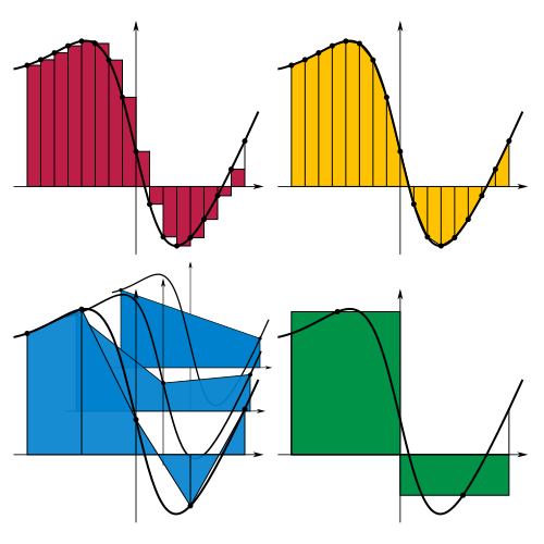
Numerical Integration Techniques for EOMs#
Euler Method (Forward Euler)#
Simple, but not very accurate
Does not conserve energy in many systems (especially oscillatory systems)
Notice that we use the acceleration at the beginning of the time step.
Numerical Integration Techniques for EOMs#
Euler-Cromer Method (Semi-Implicit Euler)#
Simple, more accurate than Euler
Conserves energy in many oscillatory systems
Notice that we use the updated velocity at the end of the time step.
Numerical Integration Techniques for EOMs#
Velocity Verlet Method#
More accurate than Euler and Euler-Cromer
Conserves energy in many oscillatory systems
Notice that we use the average acceleration over the time step. Be careful not to confuse this with your kinematic equations!
Other Common Numerical Integration Techniques for EOMs#
Runge-Kutta 2nd Order (RK2)
Runge-Kutta 4th Order (RK4)
Leapfrog Method
Beeman’s Algorithm
\(\dots\)
Many of these methods are more accurate, but also more complex to implement.
They are available in Python’s scientific computing libraries (e.g., scipy.)