
Day 09 - Modeling Drag#
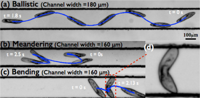
Somersault of Paramecium in extremely confined environments ->
source: https://www.nature.com/articles/srep13148
Announcements#
Homework 3 is posted (due Friday; late after Sunday)
Homework 4 is posted (due next Friday; late after Sunday)
First midterm is coming up (assigned 16 Feb)
One exercise will ask you to get started on your final project planning.
Who are you gonna work with? What are you interested in studying? Start thinking about this!
Limiting using RaiseMyHand to Workshop Days on (Fridays) only.
Will start posting the link to collect your questions for those days.
HW1 Feedback#
Overall, folks did well; some issues with uploading/submitting
Submit a regrade request if you think something was graded incorrectly
Kang has ALOT of grading to do
Grading of your HW will be completed by the Monday a week following the Sunday due date
We will not grade homework that has not been submitted properly
Delays will be handled on a case-by-case basis
Please assign problem sections to your assignment. It takes five more minutes. Please submit your assignment as a single PDF file. It makes sure your grade is correct.
Clicker Question 9-0#
I need help making sure my homework submissions are done correctly.
I think I am doing it correctly.
I am not sure if I am doing it correctly.
I know I am not doing it correctly. Please help.
If you select 2 or 3, make a mental note to please see me soon and so we can go through it together or debug your process.
Weekly Seminars#
TUESDAY, February 3, 2026#
Nuclear Theory Seminar, 11:00 a.m., FRIB 1200 Lab & Zoom Speaker: Ryan LaRose, MSU Title: Error mitigation for partially-error corrected quantum computers Zoom Link: 964 7281 4717 Passcode: 48824
Weekly Seminars#
WEDNESDAY, February 4, 2026#
Astronomy Seminar, 1:30 p.m., BPS 1400 & Zoom Speaker: Marvin Morgan, UCSB Title: TBA Zoom Link: https://msu.zoom.us/j/93334479606?pwd=OtIXPWhRPBfzYu53sl3trSJlaBYI7C.1 Passcode: 825824
Weekly Seminars#
THURSDAY, February 5, 2026#
Colloquium, Seminar, 3:30 p.m., BPS 1415 & Zoom Refreshments at 3:00 BPS in BPS 1400 Speaker: Glennys Farrar, New York University Title: Origin of ultrahigh-energy cosmic rays in Binary Neutron Star Collisions and the crucial roles of Nuclear Physics Zoom Link: https://msu.zoom.us/j/94951062663 Password: 2002
Weekly Seminars#
FRIDAY, February 6, 2026#
QuIC, Seminar, 12:40 p.m., BPS 1300 & Zoom Speaker: Gregory Quiroz, APL Title: Classical Non-Markovian Noise in Symmetry-Preserving Quantum Dynamics *For the full schedule, please see: https://sites.google.com/msu.edu/quic-seminar/ or for more information, please reach out to Ryan LaRosa directly
Reminder: Email Danny (caball14@msu.edu) your extra credit seminar write-ups
Goals for this week#
Establish a model for drag forces
Develop an understanding of the process for modeling forces
Produce equations of motion that can be investigated
Start probing the behavior of these systems with math and computing
Reminders#
Force Models#
We have been modeling the drag force using a functional dependence on velocity.
where \(f(v)\) is a function of velocity.
We established (in 1D) there are two common forms of drag force:
Reminders#
Reynolds Number#
The choice of which drag model to use depends on the Reynolds number of the system:
where \(\rho\) is the density of the fluid, \(v\) is the velocity of the object relative to the fluid, \(L\) is a characteristic linear dimension (e.g., diameter of a sphere), and \(\eta\) is the dynamic viscosity of the fluid.
Reminders#
Equations of Motion#
The next step is to use Newton’s 2nd Law to write the equations of motion for the system. We found those equation of motion to be:
where \(f(v)\) is the drag force. So for each form of drag we have:
Reminders#
Trajectories#
We can integrate these equations of motion to find the velocity as a function of time. We found:
where \(v_{\text{t,lin}} = \frac{mg}{b}\) for linear drag and \(v_{\text{t,quad}} = \sqrt{\frac{mg}{c}}\) for quadratic drag.
Our Current Investigatory Process#
The Model-to-Trajectory Pipeline#
Model the forces acting on the system
Write the equations of motion using Newton’s 2nd Law
Solve the equations of motion to find trajectories
This is incomplete. We will need to learn how stability, critical points, and phase space can help us understand the behavior of these systems.
We have also only done step 3 analytically. We will need to learn how to use computing to investigate these systems.
Clicker Question 9-1#
The Reynolds number can be thought of as a comparison between two forces acting on an object moving through a fluid: (1) inertial forces and (2) viscous forces. The ratio gives a sense of which force dominates the behavior of the object.
Clicker Question 9-1#
With this in mind, consider again the Reynolds number formula:
Consider three scenarios:
A person swimming through water at moderate speed.
A small bacterium swimming through water at low speed.
A large airplane flying through the air at high speed.
Order these scenarios from lowest to highest Reynolds number.
1. 1, 3, 2; 2. 2, 3, 1; 3. 1, 2, 3, 4. 3, 1, 2; 5. Something else
Clicker Question 9-2#
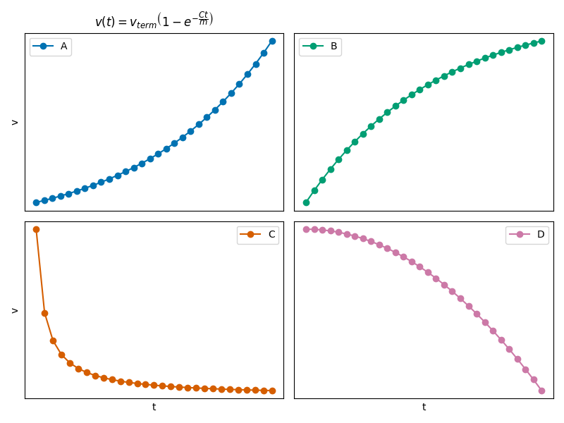
For the system of Linear Drag in 1D, we found a solution for the velocity as a function of time, with \(v = 0\) at \(t = 0\). $\(v(t) = v_{term}\left(1-e^{-\frac{bt}{m}}\right)\)$
where \(v_{term} = \sqrt{\frac{mg}{b}}\).
Which sketch could be correct for the velocity of the ball?
Clicker Question 9-3#
For the system of Quadratic Drag in 1D, we found a solution for the velocity as a function of time, with \(v = 0\) at \(t = 0\).
where \(v_{term} = \sqrt{mg/c}\). What happens when \(t \rightarrow \infty\)?
The object stops moving.
The object travels at a constant velocity.
The object travels at an increasing velocity.
The object travels at a decreasing velocity.
I’m not sure.
Clicker Question 9-4#
For quadratic drag in 2D, we found the following pair of differential equations:
True or False: This pair of differential equations can be decoupled.
True
False
???
Clicker Question 9-5#
For linear drag in 2D, we found the following pair of differential equations:
True or False: This pair of differential equations is decoupled.
True
False
???
Clicker Question 9-6#
For the gravitational interaction, I want to compute the force acting on body B, located at \(\vec{r}_B\), by body A, located at \(\vec{r}_A\).
The gravitational force is given by:
What is the appropriate form of \(\vec{r}\)?
\(\vec{r} = \vec{r}_A - \vec{r}_B\)
\(\vec{r} = \vec{r}_B - \vec{r}_A\)
Either is ok
Clicker Question 9-7#
We found that the equation of motion for the spring-mass system was:
Your friends have proposed the following general solutions:
How many of them are correct? (1) Only one (2) Two (3) Three (4) Four (5) All of them