
Day 27 - Introduction to Chaos#
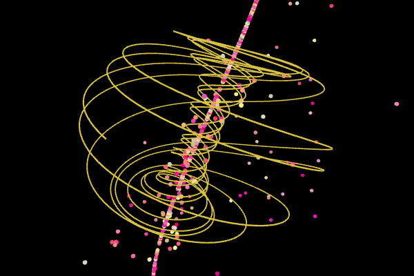
Sprott Attractor#
Announcements#
Midterm 1 (problems 2 and 3) is graded
Problem 1 is still being graded
Homework 7 is due Friday
No homework next week
Midterm 2 will be assigned next Monday (due 18 April)
Second project check-in
Seminars This Week#
MONDAY, March 24, 2025#
Condensed Matter Seminar 4:10 pm, 1400 BPS, Andrew Kirkpatrick, MSU, Fabrication of orientated NV centres in diamond by ultrafast laser fabrication AND Ankang Liu, MSU Effect of hole-strain coupling on the eigenmodes of semiconductor-based nanomechanical systems
Seminars This Week#
WEDNESDAY, March 26, 2025#
Astronomy Seminar, 1:30 pm, 1400 BPS, Bryan Terrazas, Oberlin College, Galaxy evolution and feedback modeling
FRIB Nuclear Science Seminar, 3:30pm., FRIB 1300 Auditorium, Dr. Jacklyn Gates of Lawrence Berkeley National Laboratory, Toward Pursuing New Superheavy Elements
Seminars This Week#
THURSDAY, March 27, 2025#
Special FRIB/MSU Nuclear Science Seminar with Colloquium, 3:30 pm, 1415 BPS, Mandie Gehring, LANL, Measuring Intense X-ray Spectra and an Overview of Space Research at Los Alamos National Laboratory
FRIDAY, March 28, 2025#
IReNA Online Seminar, 2:00 pm, In Person and Zoom, FRIB 2025 Nuclear Conference Room, Jordi José, Technical University of Catalonia, UPC (Barcelona, Spain), Classical novae at the crossroads of nuclear physics, astrophysics and cosmochemistry
What is Chaos?#

At your table, discuss what it means for a system to be chaotic.
What are some examples of chaotic systems?
What are some characteristics of chaotic systems?
How do chaotic systems differ from non-chaotic systems?
Try to come up with two answers to each question to share.
Hallmarks of a Classically Chaotic System#
Deterministic: The system is governed by deterministic laws (e.g., Newton’s laws of motion, a set of differential equations)
Sensitive to Initial Conditions: A bundle of trajectories that start close together will diverge exponentially over time
Non-periodic Behavior: The system exhibist s complex, non-repeating behavior over time, this might look like “random” behavior, but it is not truly random because it is deterministic
Hallmarks of a Classically Chaotic System#
Strange Attractors: The system may have a strange attractor, which is a fractal structure in phase space that the system tends to evolve towards over time
Parameter Sensitivity: The system may be sensitive to small changes in parameters, which can trigger qualitative changes in the system’s behavior
(Sometimes) Periodic Behavior: The system may exhibit periodic behavior for certain parameter values, and this might be a signal that the system bifurcates into chaotic behavior for other parameter values
Example 1: Duffing Equation#
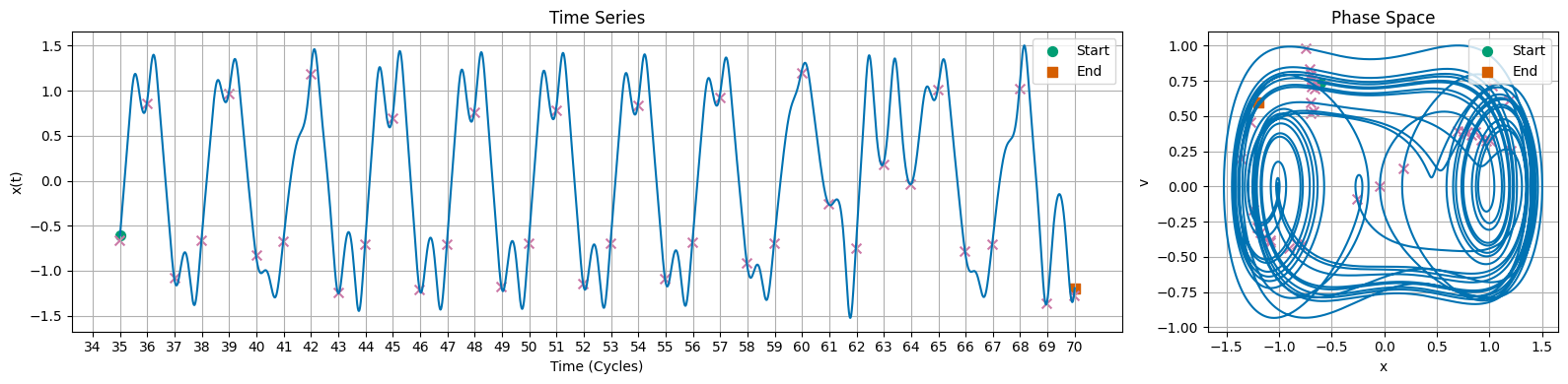
Exhibits Periodic and Chaotic Behavior
Illustrates period doubling bifurcations as route to chaos
Example 2: Lorenz System#
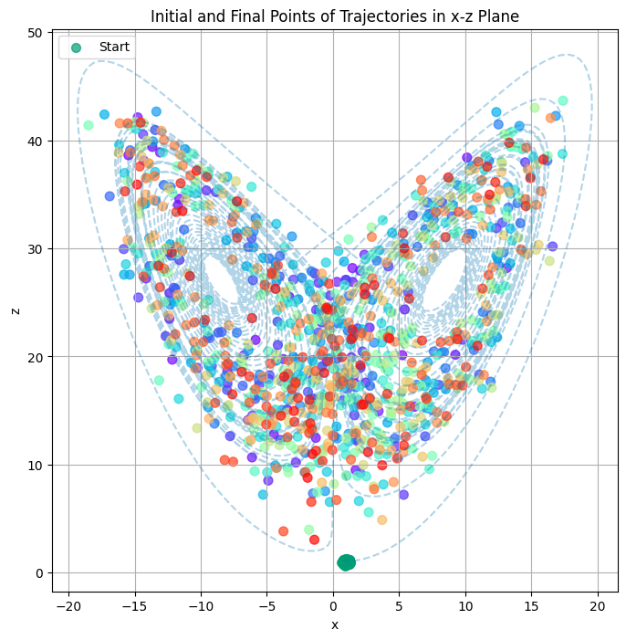
Exhibits sensitive dependence on initial conditions Demonstrates the concept of a strange attractor
Using solve_ivp#
We will start with the damped driven pendulum as an example. This will illustrate how to use solve_ivp to solve a system of coupled first-order differential equations.
We can rewrite this as two first-order equations:
Using solve_ivp#
To use solve_ivp, we write a function for the derivatives:
def damped_driven_pendulum(t, y, beta, A, omegaD=1):
    theta, omega = y
    dtheta_dt = omega
    domega_dt = -np.sin(theta) - beta * omega + A * np.cos(omegaD*t)
    return [dtheta_dt, domega_dt]
Using solve_ivp#
Now we can use solve_ivp to solve the system of equations:
# Parameters that define the system
beta = 0.5
A = 1.0
omegaD = 2*np.pi

# Time span for the simulation
t_span = (0, 100)

# Initial conditions: [theta, omega]
y0 = [6, 0]

# Time points where we want the solution
t_eval = np.linspace(t_span[0], t_span[1], 10000)

# Solve the system of equations
solution = solve_ivp(damped_driven_pendulum, t_span, y0, args=(beta, A, omegaD), t_eval=t_eval)
Damped Driven Pendulum#
Long Term Behavior is Periodic
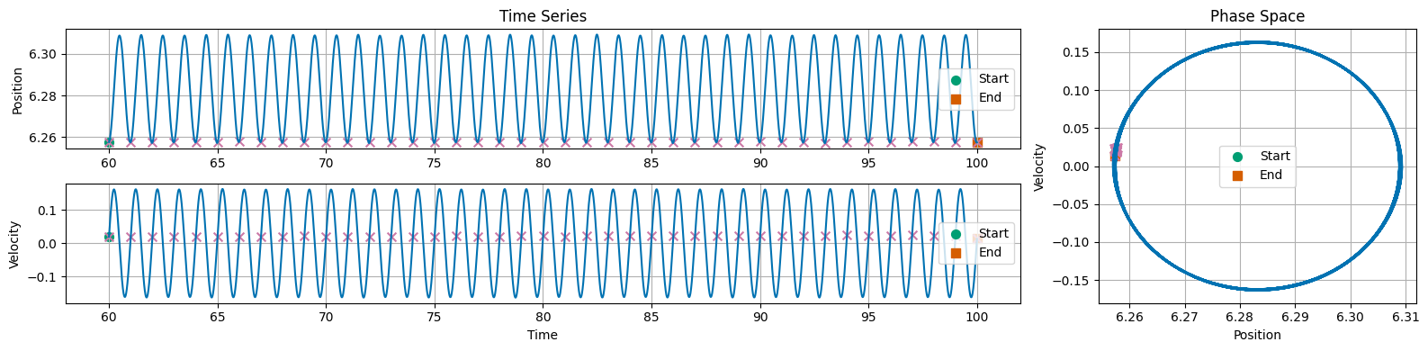
“Period-1” Dynamics is a term to indicate there’s a single frequency governing the motion
Phase space plots can provide a better window into the system’s behavior