
Day 26 - Introduction to Chaos#
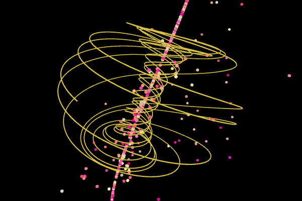
https://www.dynamicmath.xyz/strange-attractors/
Announcements#
Midterm 1 is graded
Feedback delivered for project
Still some outstanding grading issues
Homework 7 is due Friday
No homework next week
Midterm 2 will be assigned next Monday
Second project check-in
What is Chaos?#

At your table, discuss what it means for a system to be chaotic.
What are some examples of chaotic systems?
What are some characteristics of chaotic systems?
How do chaotic systems differ from non-chaotic systems?
Try to come up with two answers to each question to share.
Hallmarks of a Classically Chaotic System#
Deterministic: The system is governed by deterministic laws (e.g., Newton’s laws of motion, a set of differential equations)
Sensitive to Initial Conditions: A bundle of trajectories that start close together will diverge exponentially over time
Non-periodic Behavior: The system exhibist s complex, non-repeating behavior over time, this might look like “random” behavior, but it is not truly random because it is deterministic
Hallmarks of a Classically Chaotic System#
Strange Attractors: The system may have a strange attractor, which is a fractal structure in phase space that the system tends to evolve towards over time
Parameter Sensitivity: The system may be sensitive to small changes in parameters, which can trigger qualitative changes in the system’s behavior
(Sometimes) Periodic Behavior: The system may exhibit periodic behavior for certain parameter values, and this might be a signal that the system bifurcates into chaotic behavior for other parameter values
Example 1: Duffing Equation#
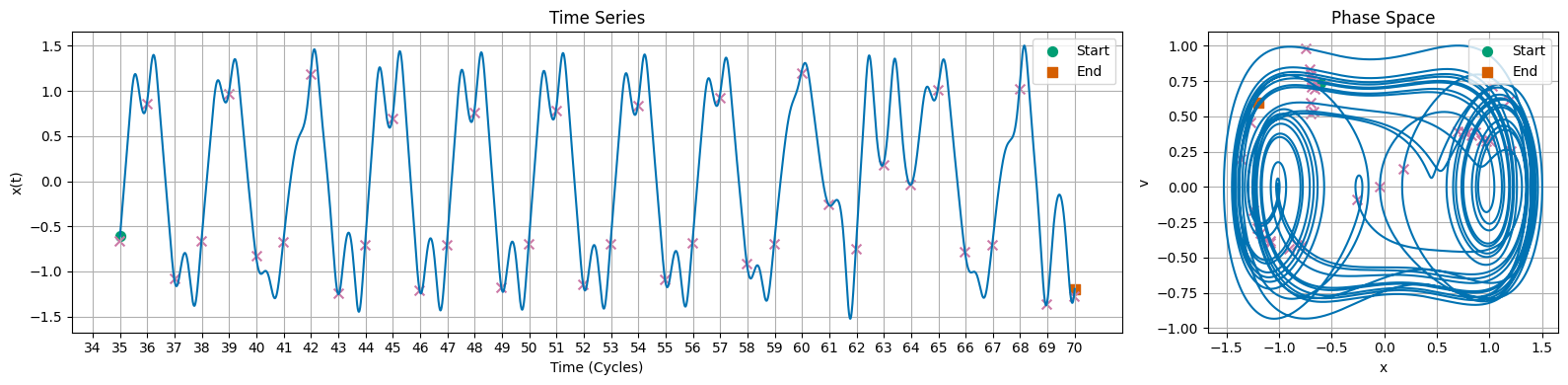
Exhibits Periodic and Chaotic Behavior
Illustrates period doubling bifurcations as route to chaos
Example 2: Lorenz System#
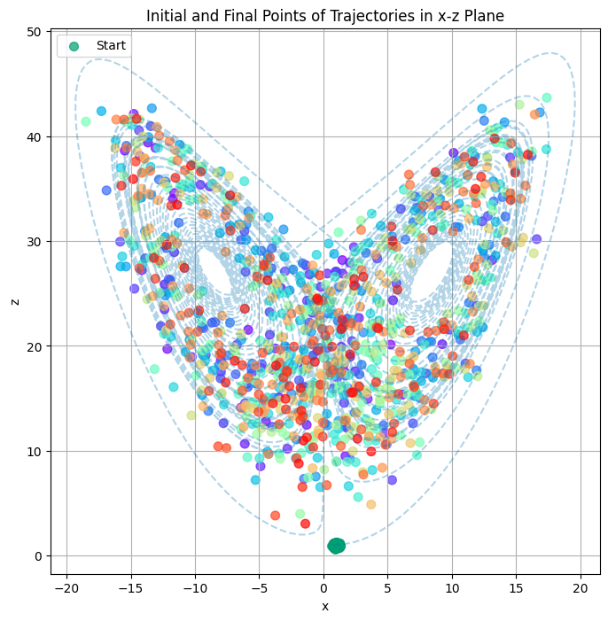
Exhibits sensitive dependence on initial conditions Demonstrates the concept of a strange attractor
Using solve_ivp#
We will start with the damped driven pendulum as an example. This will illustrate how to use solve_ivp to solve a system of coupled first-order differential equations.
We can rewrite this as two first-order equations:
Using solve_ivp#
To use solve_ivp, we write a function for the derivatives:
def damped_driven_pendulum(t, y, beta, A, omegaD=1):
    theta, omega = y
    dtheta_dt = omega
    domega_dt = -np.sin(theta) - beta * omega + A * np.cos(omegaD*t)
    return [dtheta_dt, domega_dt]
Using solve_ivp#
Now we can use solve_ivp to solve the system of equations:
# Parameters that define the system
beta = 0.5
A = 1.0
omegaD = 2*np.pi

# Time span for the simulation
t_span = (0, 100)

# Initial conditions: [theta, omega]
y0 = [6, 0]

# Time points where we want the solution
t_eval = np.linspace(t_span[0], t_span[1], 10000)

# Solve the system of equations
solution = solve_ivp(damped_driven_pendulum, t_span, y0, args=(beta, A, omegaD), t_eval=t_eval)
Damped Driven Pendulum#
Long Term Behavior is Periodic
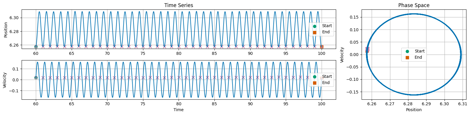
“Period-1” Dynamics is a term to indicate there’s a single frequency governing the motion
Phase space plots can provide a better window into the system’s behavior