
Day 18 - Phase Diagrams#
Synchronization of oscillators#
Announcements#
Midterm 1 is due Feb 27th (late on March 1st)
Friday’s class: Midterm 1 discussion and support session. Bring your questions.
Seminars this week#
WEDNESDAY, February 25, 2026#
Astronomy Seminar, 1:30 p.m., BPS 1400 & Zoom Speaker: Juliette Becker, University of Wisconsin-Madison Title: TBA Zoom Link: https://msu.zoom.us/j/93334479606?pwd=OtIXPWhRPBfzYu53sl3trSJlaBYI7C.1 Passcode: 825824
WEDNESDAY, February 25, 2026#
FRIB Nuclear Science Seminar, 3:30 p.m., FRIB 1300 & Zoom Speaker: Jordan Stomps, Oak Ridge National Laboratory Title: Data Science and Engineering for Nuclear Nonproliferation Zoom Link: https://msu.zoom.us/j/93742845358?pwd=vlen3rlRdk8NHBSOxVIM1Aj2cP144m.1 Passcode: 416741
THURSDAY, February 26, 2026#
Colloquium, Seminar, 3:30 p.m., BPS 1415 & Zoom Refreshments at 3:00 BPS in BPS 1400 Speaker: Dylan Yost, Colorado State Title: Precision tests of quantum electrodynamics through hydrogen spectroscopy and vacuum birefringence Zoom Link: https://msu.zoom.us/j/94951062663 Password: 2002 *For more information and scheduling a time to meet with the speaker, please see the calendar: https://pa.msu.edu/news-events-seminars/colloquium-schedule.aspx
FRIDAY, February 27, 2026#
QuIC, Seminar, 12:40 p.m., BPS 1300 & Zoom Speaker: Kevin Sung, IBM Title: Enhancing Chemistry on Quantum Computers with Fermionic Linear Optical Simulation *For the full schedule, please see: https://sites.google.com/msu.edu/quic-seminar/ or for more information, please reach out to Ryan LaRosa directly
FRIDAY, February 27, 2026#
IReNA Online Seminar, 2:00 pm, Zoom Light refreshments at 1:50pm in 2025 Nuclear Conference Room - FRIB Hosted by: Aldana Grichener (University of Arizona & Observatory) Speaker: Shivani Shah, North Carolina State University Title: Actinide Abundances, Variation, and Evolution in Metal-Poor Stars Zoom Link: https://msu.zoom.us/j/827950260 Password: CENAM
Reminders: Flow on a Line#
A first order ODE of the form:
can be thought of as a flow on a line. We can graph the function \(f(x)\) in the \(x\)-\(\dot{x}\) plane. Thus,
So that,
Reminders: Flow on a Line#
Example \(\dot{x} = \sin{x}\)#
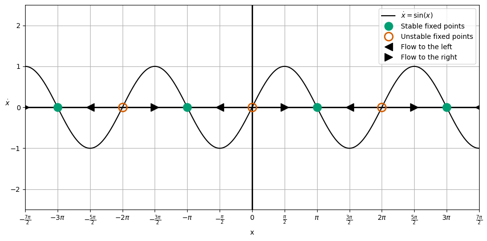
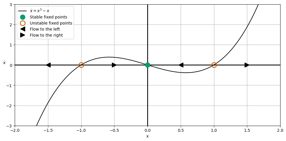
Reminders: Flow on a Line#
Example \(\dot{x} = x^3-x\)#
Firefly Synchronization#
Ermentrout and Rinzel (1984) developed a model for firefly flashing.
The basic model suggests that a firefly will flash regularly without stimulus (\(\dot{\theta} = \omega_f\)).
With a flashing stimulus that flashes at its own rate (\(\dot{\Theta} = \Omega_s\)), the firefly will attempt to synchronize with the stimulus.
That model is given by
where the \(\phi\) is the difference in the phases (\(\theta\), firefly; \(\Theta\), stimulus) is critical to the model as is the ability of the firefly to synchronize is given by \(A\).
Firefly Synchronization#
It is typical to rescale nonlinear equations to seek natural units. In this case, we choose a dimensionless time,
and a dimensionless phase difference,
Which gives the dimensionless equation for the phase difference \(\phi = \Theta - \theta\):,
Clicker Question 18-1#
Consider the dimensionless equation for the phase difference \(\phi = \Theta - \theta\):
Use the phase space of \(\phi\) vs. \({d\phi}/{d\tau}\) to sketch the phase diagram for the system. Find the equilibrium points and their stability. Consider the 3 cases.
Assume \(\mu = 0\).
Assume \(0 < \mu < 1\).
Assume \(\mu > 1\).
Click when you and your table are done.
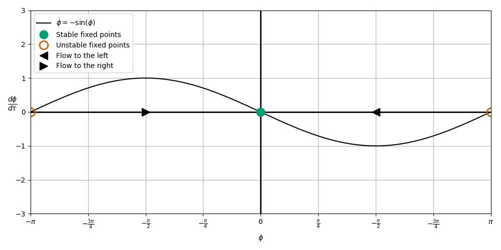
\(\mu = 0\)#
Synchronization always (no phase difference)#
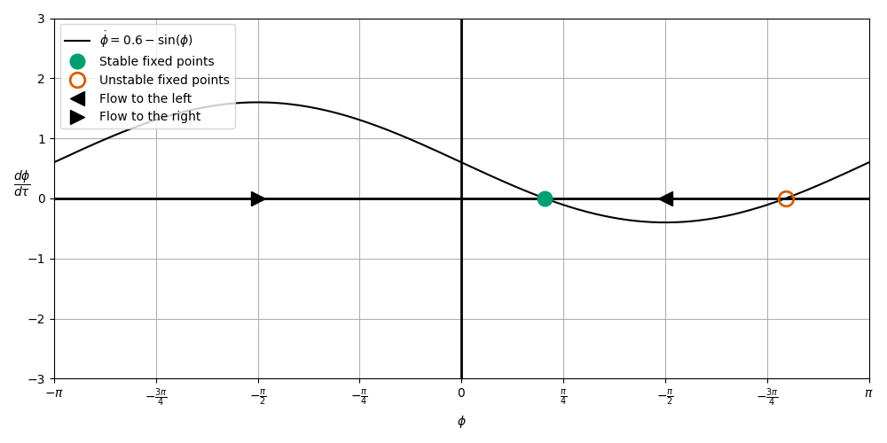
\(\mu = 0.6\)#
Entrainment is possible (constant phase difference)#
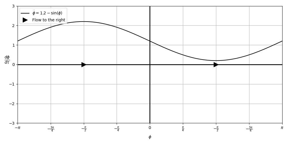
\(\mu=1.2\)#
No entrainment (\(\Omega > \omega\)). Stimulus is too fast.#
Why Fireflies?#
The firefly model is a good example of a system that can be modeled with a phase diagram.
It also has a parameter (\(\mu\)) that can be varied to change the system behavior.
The parameter \(\mu\) can be thought of as a “bifurcation parameter.”
A bifurcation is a change in the number or stability of equilibria as a parameter is varied.
It also illustrates the concept of “phase locking”, which is important in many spaces (e.g., lasers, Josephson junctions, etc.).
2D Phase Spaces#
What happens when we have differential equations that are not first order?
We can convert this to a system of first order equations by defining a new variable \(v = \dot{x}\). Then we have a system of two first order equations:
We can still use the phase space method to analyze the system in the \((x, v)\) plane.
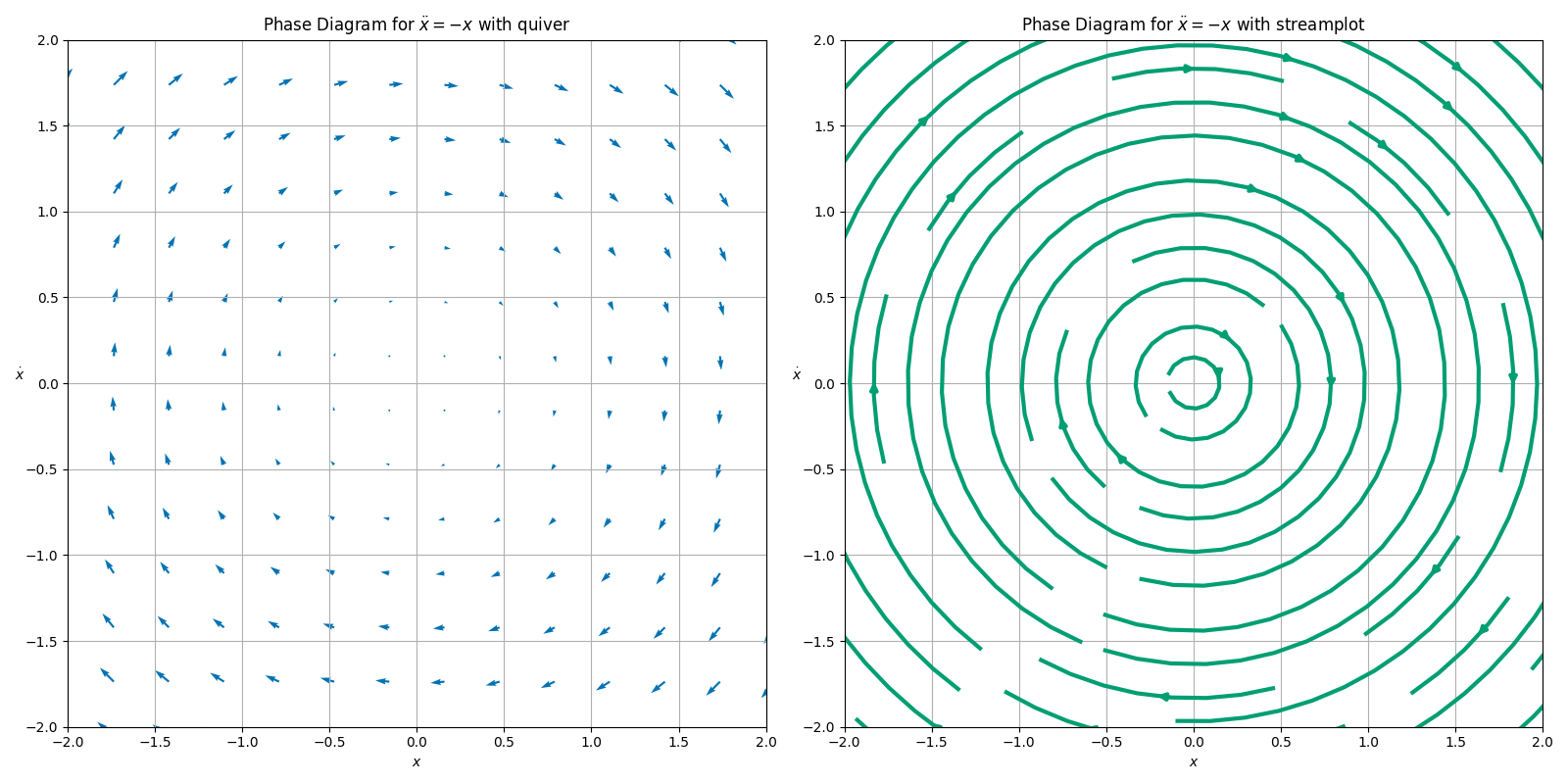
Reminders: Phase Space and the Harmonic Oscillator#
Assume a dimensionless harmonic oscillator: $\(\ddot{x} = -x\)$
We convert this to a system of first order equations:
We can graph the system in the \((x, v)\) plane.
Steps for a Sketching a 2D Phase Diagram#
Seperate the system into two first order equations.
At each point \((x, v)\), find the vector \(\langle \dot{x}, \dot{v} \rangle\).
Represent this vector as an arrow in the \((x, v)\) plane. This gives the “flow field” of the phase space.
Continue this process until you have a good representation of the flow field.
Hint: Start with points that are easy to sketch. But we will eventually use a computer to do this.
Clicker Question 18-2#
Consider the pair of first order equations:
Choose the \(x=0\) line; the vertical axis.
Note that there will only be horizontal arrows on this line. Why?
Sketch the arrows on the \(x=0\) line.
Click when you and your table are done.
Clicker Question 18-3#
Now, SEPERATELY, please do this separately lest we draw historical symbols that we should not. Fascism has no home here, y’all.
Choose the \(v=0\) line; the vertical axis.
Note that there will only be vertical arrows on this line. Why?
Sketch the arrows on the \(v=0\) line.
Click when you and your table are done.
Clicker Question 18-4#
Now try another line, the \(x=\pm v\) line.
Choose a diagonal line, \(x=v\). $\(\langle \dot{x}, \dot{v} \rangle = \langle v, -v \rangle\)$
Sketch the arrows on the \(x=v\) line.
Choose a diagonal line, \(x=-v\).
Sketch the arrows on the \(x=-v\) line.
Connect the arrows to represent the flow field as closed loops.
Click when you and your table are done.
Flow field for the harmonic oscillator#
Clicker Question 18-5#
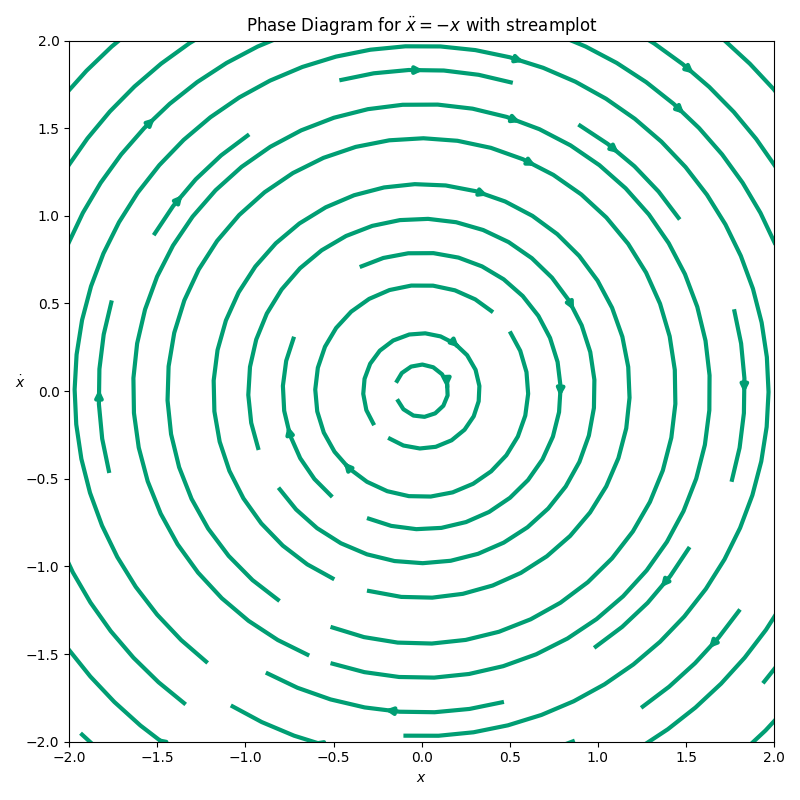
What shape are the arrows tracing out in the phase space for the harmonic oscillator?
A circle
An ellipse
Annoying sibling voice: “A circle is an ellipse, dummy”
We don’t talk like that to each other. 🥰
A spiral?
Clicker Question 18-6#
These curves never touch, why is that? What does a closed curve in this phase space represent?
The motion is orbital
The motion is periodic.
The system has constant energy.
The system’s energy changes throughout.
More than one of the above.