
Day 17 - Nonlinear Dynamics#
Rössler Attractor#
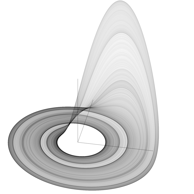
There are no crossings of the path shown in this picture#
Announcements#
Midterm 1 is due Feb 27th (late on March 1st)
Friday’s class: Midterm 1 discussion and support session. Bring your questions.
Seminars this week#
MONDAY, February 23, 2026#
Condensed Matter Physics Seminar, 4:10p.m., BPS 1400 & Zoom Speaker: Ilija Zeljkovic, Boston College Title: Atomic-scale imaging of symmetry-broken electronic states in kagome superconductors Zoom Link: https://msu.zoom.us/j/93613644939 Password: CMP
TUESDAY, February 24, 2026#
High Energy Physics Seminar, 1:30p.m., BPS 1400 & Zoom Speaker: Daniel Adamiak/Artemiy Filippov, MSU Title: Investing the phenomenon of double descent in cross-validation *For the Zoom link – Please contact Joey Huston, Sophie Berkman and/or Brenda Wenzlick
WEDNESDAY, February 25, 2026#
Astronomy Seminar, 1:30 p.m., BPS 1400 & Zoom Speaker: Juliette Becker, University of Wisconsin-Madison Title: TBA Zoom Link: https://msu.zoom.us/j/93334479606?pwd=OtIXPWhRPBfzYu53sl3trSJlaBYI7C.1 Passcode: 825824
WEDNESDAY, February 25, 2026#
FRIB Nuclear Science Seminar, 3:30 p.m., FRIB 1300 & Zoom Speaker: Jordan Stomps, Oak Ridge National Laboratory Title: Data Science and Engineering for Nuclear Nonproliferation Zoom Link: https://msu.zoom.us/j/93742845358?pwd=vlen3rlRdk8NHBSOxVIM1Aj2cP144m.1 Passcode: 416741
THURSDAY, February 26, 2026#
Colloquium, Seminar, 3:30 p.m., BPS 1415 & Zoom Refreshments at 3:00 BPS in BPS 1400 Speaker: Dylan Yost, Colorado State Title: Precision tests of quantum electrodynamics through hydrogen spectroscopy and vacuum birefringence Zoom Link: https://msu.zoom.us/j/94951062663 Password: 2002 *For more information and scheduling a time to meet with the speaker, please see the calendar: https://pa.msu.edu/news-events-seminars/colloquium-schedule.aspx
FRIDAY, February 27, 2026#
QuIC, Seminar, 12:40 p.m., BPS 1300 & Zoom Speaker: Kevin Sung, IBM Title: Enhancing Chemistry on Quantum Computers with Fermionic Linear Optical Simulation *For the full schedule, please see: https://sites.google.com/msu.edu/quic-seminar/ or for more information, please reach out to Ryan LaRosa directly
FRIDAY, February 27, 2026#
IReNA Online Seminar, 2:00 pm, Zoom Light refreshments at 1:50pm in 2025 Nuclear Conference Room - FRIB Hosted by: Aldana Grichener (University of Arizona & Observatory) Speaker: Shivani Shah, North Carolina State University Title: Actinide Abundances, Variation, and Evolution in Metal-Poor Stars Zoom Link: https://msu.zoom.us/j/827950260 Password: CENAM
Reminders: Conservative Forces#
The curl of a conservative force is zero
Work done by a conservative force is path-independent
Work done by a conservative force around a closed path is zero
Reminders: Conservative Forces#
The work done by a conservative force is equal to the negative of the change in potential energy
A conservative force can be expressed as the gradient of a scalar function
Reminders: Equilibrium (aka Critical or Fixed) Points#
We found equilibrium points by setting the derivative of the potential energy to zero:
We then determined if these points were stable or unstable by looking at the second derivative of the potential energy:
Relationship to Differential Equations#
By setting \(\frac{dU}{dx} = 0\), we are finding the equilibrium points where the force is zero,
If we consider the typical form of a differential equation, we can see that we are seeking the points where the differential equation is zero,
This approach is a powerful way to understand the behavior of a system. And we can do so geometrically!
Clicker Question 17-1#
Let \(\dot{x}=\sin{x}\). Set up the integral that could be used to solve for \(t(x)\).
\(\int \frac{dx}{\sin{x}}\)
\(\int \frac{dx}{\cos{x}}\)
\(\int \frac{dx}{\tan{x}}\)
\(\int \frac{dx}{\cot{x}}\)
???
Clicker Question 17-2#
We can integrate this with \(x(0)=x_0\) to find \(t(x)\):
Find \(x(t)\)? 🤢🤢🤢
Instead find the equilibrium points (\(x^*\)) of the system. \(n\) is an integer.
\(x^*=0\)
\(x^*=0, \pm\pi\)
\(x^*=\pm\pi/2\)
\(x^*=n\frac{\pi}{2}\)
\(x^*=n\pi\)
Clicker Question 17-3a#
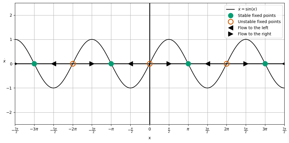
Sketch the differential equation \(\dot{x} = \sin{x}\) in the phase space \(x\) vs. \(\dot{x}\).
Note where the plot crosses the \(x\)-axis. These are the critical/equilibrium points, \(x^*\). Identify the critical points.
By definition, \(\dot{x} > 0\) is a “flow to the right” and \(\dot{x} < 0\) is a “flow to the left”. Sketch the direction of the flow - this should only appear in the \(x\)-axis.
Click when you and your table are done.
Clicker Question 17-3b#
Sketch the differential equation \(\dot{x} = \sin{x}\) in the phase space \(x\) vs. \(\dot{x}\).
Look at the flow directions and the critical points. What can you say about the stability of the critical points? We use closed circles for stable points and open circles for unstable points. Add these to your plot.
Click when you and your table are done.
Phase Space Diagram for \(\dot{x} = \sin{x}\)#
Clicker Question 17-4a#
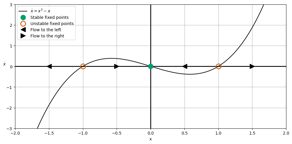
Consider now the differential equation \(\dot{x} = x^3 - x\). To find \(t(x)\), we can integrate:
That yields the following solution (🤢🤢🤢):
Find the equilibrium points (\(x^*\)) of the system.
Sketch the differential equation \(\dot{x} = x^3 - x\) in the phase space \(x\) vs. \(\dot{x}\).
Click when you and your table are done.
Clicker Question 17-4b#
Consider now the differential equation \(\dot{x} = x^3 - x\). To find \(t(x)\), we can integrate:
That yields the following solution (🤢🤢🤢):
What can you say about the stability of the critical points? Add these to your plot.
Click when you and your table are done.
Phase Space Diagram for \(\dot{x} = x^3 - x\)#
The Harmonic Oscillator Gets a Bad Rap#
The SHO is a linear system. It’s boring. It’s predictable. It’s stable. But it can help us understand nonlinear 2nd order ODEs and thus more complex systems.
Consider the physical pendulum. The equation of motion is
Or more simply:
In the case of small angles, \(\sin{\theta} \approx \theta\), and we have a linear system.
Examples of SHOs#
The spring-mass system \(\ddot{x} = -\omega^2 x\)
The simple pendulum \(\ddot{\theta} = -\frac{g}{L}\theta\)
The LC circuit \(\ddot{q} = -\frac{1}{LC}q\)
Water in a u-tube \(\ddot{h} = -\frac{2g\rho A}{M}h\)
A jump rope \(\ddot{u} = \frac{T}{\lambda}\left(\frac{n\pi}{d}\right)^2 u\)
Any system with a local minimum in the potential energy can ber modeled as an SHO.