Numerically Integrating the SHO model

import numpy as np
import matplotlib.pyplot as plt

%matplotlib inline

a = 1 
print(a)

1

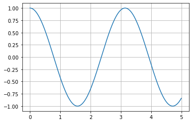
x0 = 1.0 ## Initial position
v0 = 0.0 ## Initial velocity

omega = 2 ## Angular freq. of SHO

tf = 5 ## Model time

def AnalyticalSolutionSHO(tf, deltat, amp, omega, t0 = 0, phase = 0):
    
    if t0 < tf:
        
        t = np.arange(t0,tf,deltat) ## equal steps
        x = amp*np.cos(omega*t+phase)
        
        return t,x
    
    else:
        
        raise ValueError('Final time is before start time.')

deltat = 0.001
t,x = AnalyticalSolutionSHO(tf, deltat, x0, omega)
plt.plot(t,x)
plt.grid()

\[\ddot{x} = -\omega x\]

\[\dfrac{d^2x}{dt^2} = -\omega x\]

Introduce \(u=\dot{x}\), so that \(\dot{u}=\ddot{x}\). We can produce two coupled, linear, first order, ODEs:

\[\dot{u} = -\omega x\]

\[\dot{x} = u\]

Imagine we allow ourselves to take a small step in time \(\Delta t\), how would \(u\) and \(x\) change in that time?

\[\dot{x} = \dfrac{dx}{dt} = \lim_{\Delta t \rightarrow 0} \dfrac{x(t+\Delta t) - x(t)}{\Delta t} = u\]

So that,

\[x(t+\Delta t) \approx u\Delta t + x(t)\]

Similarly, $\(u(t+\Delta t) \approx -\omega x \Delta t + u(t)\)$

Developing a Numerical Routine

Notice we have two equations that describe how to obtain new values of location (\(x\)) and velocity (\(u\)) at a time \(t+\Delta t\) given information about the system at some earlier time, \(t\), (or at the least, considering the location and velocity at time \(t\)), which we take as a pair of update equations where the equality holds:

\[x(t+\Delta t) = u\Delta t + x(t)\]

\[u(t+\Delta t) = -\omega x \Delta t + u(t)\]

That is, they can potentially tell us at least in a short time \(\Delta t\) that we can estimate the velocity (\(u\)) and location (\(x\)) of the oscillator. We have not shown these can be used repeatedly to produce an estimated trajectory yet. As you might expect, these are better update equations when \(\Delta t\) is small. But there’s another ambiguity:

\[x(t+\Delta t) = \underbrace{u}_{\mathtt{?}}\Delta t + x(t)\]

\[u(t+\Delta t) = -\omega \underbrace{x}_{\mathtt{?}} \Delta t + u(t)\]

The quantities with the underbrace are ambiguous. Do we use the values of \(x\) and \(u\) at a time \(t\), \(t+\Delta t\), or something else?!

The choice matters

Let’s illustrate this with making different choices using the following routine:

Basic ODE Integration Routine

initialCond0 = VAL0
initialCond1 = VAL1
...
initialCondN = VALN

startTime = START
stopTime = STOP
steps =  STEPS
deltaT = (stopTime-startTime)/steps

t = startTime

while t < stopTime:

    updatedVal0 = updateEqn0()
    updatedVal1 = updateEqn1()
    ...
    updatedValN = updateEqnN()
    
    store(updatedVals)
    
    t += deltaT

This might seem quite abstract, so let’s make a table of choices for our integration routines:

Approach	Value of x	Value of u	Considerations
1	\(x(t)\)	\(u(t)\)	We have both of these values to start
2	\(x(t)\)	\(u(t+\Delta t)\)	For this, we will need a \(u(t+\Delta t)\) estimate first
3	\(x(t+\Delta t)\)	\(u(t)\)	Hmm…we will need a \(x(t+\Delta t)\) estimate first
4	\(x(t+\Delta t)\)	\(u(t+\Delta t)\)	Well this doesn’t seem possible to get both estimates at the same time!

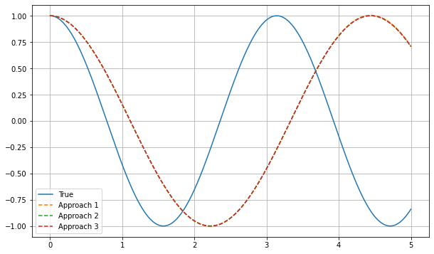
It looks like we can try approach 1, 2, and 3 without much fuss. Let’s write a few functions.

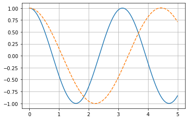
N = int(np.ceil(tf/deltat))
steps = np.arange(0, N-1)
deltaT = tf/N
time = np.linspace(0,tf,N)

##Approach 1
xVals1 = np.zeros(N)
uVals1 = np.zeros(N)

xVals1[0] = x0
uVals1[0] = v0

for i in steps:
    
    uVals1[i+1] = uVals1[i] + xVals1[i]*deltaT
    xVals1[i+1] = xVals1[i] - omega*uVals1[i]*deltaT

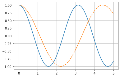
plt.plot(t, x)
plt.plot(time, xVals1, '--')
plt.grid()

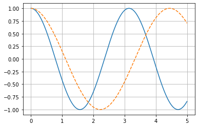
## Approach 2

xVals2 = np.zeros(N)
uVals2 = np.zeros(N)

xVals2[0] = x0
uVals2[0] = v0

for i in steps:
    
    uVals2[i+1] = uVals2[i] + xVals2[i]*deltaT
    xVals2[i+1] = xVals2[i] - omega*uVals2[i+1]*deltaT

plt.plot(t, x)
plt.plot(time, xVals2, '--')
plt.grid()

## Approach 3

xVals3 = np.zeros(N)
uVals3 = np.zeros(N)

xVals3[0] = x0
uVals3[0] = v0

for i in steps:
    
    xVals3[i+1] = xVals3[i] - omega*uVals3[i]*deltaT
    uVals3[i+1] = uVals3[i] + xVals3[i+1]*deltaT

plt.plot(t, x)
plt.plot(time, xVals3, '--')
plt.grid()

plt.figure(figsize=(10,6))
plt.plot(t, x)
plt.plot(time, xVals1, '--')
plt.plot(time, xVals2, '--')
plt.plot(time, xVals3, '--')
plt.legend(['True', 'Approach 1', 'Approach 2', 'Approach 3'])
plt.grid()

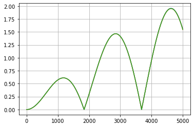
plt.plot(np.abs(x-xVals1))
plt.plot(np.abs(x-xVals2))
plt.plot(np.abs(x-xVals3))
plt.grid()

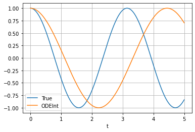
from scipy.integrate import odeint

def NumericalSolutionSHO(y, t, omega):
    
    x, vx = y
    dydt = [vx, -omega*x]
    return dydt

omega0 = omega
y0 = [x0, v0]
t = time
sol = odeint(NumericalSolutionSHO, y0, t, args=(omega0,))

plt.plot(t, x, label='True')
plt.plot(t, sol[:,0], label='ODEInt')
plt.legend(loc='best')

plt.xlabel('t')

plt.grid()