
5. Harmonic Oscillations#
The harmonic oscillator is omnipresent in physics. Although you may think of this as being related to springs, it, or an equivalent mathematical representation, appears in just about any problem where a mode is sitting near its potential energy minimum. At that point, \(\partial_x V(x)=0\), and the first non-zero term (aside from a constant) in the potential energy is that of a harmonic oscillator. In a solid, sound modes (phonons) are built on a picture of coupled harmonic oscillators, and in relativistic field theory the fundamental interactions are also built on coupled oscillators positioned infinitesimally close to one another in space. The phenomena of a resonance of an oscillator driven at a fixed frequency plays out repeatedly in atomic, nuclear and high-energy physics, when quantum mechanically the evolution of a state oscillates according to \(e^{-iEt}\) and exciting discrete quantum states has very similar mathematics as exciting discrete states of an oscillator.
Harmonic Oscillator, deriving the Equations#
The potential energy for a single particle as a function of its position \(x\) can be written as a Taylor expansion about some point \(b\) (we are considering a one-dimensional problem here)
If the position \(b\) is at the minimum of the resonance, the first two non-zero terms of the potential are
Our equation of motion is, with the only force given by the one-dimensional spring force,
Defining the natural frequency \(\omega_0^2=k/m\) we can rewrite this equation as
We call this a natural frequency since it is defined by the constants that describe our system, the spring constant \(k\) and the mass \(m\) of the object.
We can as usual split this equation of motion into one equation for the derivative of the velocity and
and
The solution to the equations of motion is given by
where \(A\) and \(B\) are in general complex constants to be determined by the initial conditions.
Inserting the solution into the equation of motion we have
we have
and the right-hand side is just \(-\omega_0^2 x(t)\). Thus, inserting the solution into the differential equation shows that we obtain the same original differential equation.
Let us assume that our initial time \(t_0=0\)s and that the initial position \(x(t_0)=x_0\) and that \(v_0=0\) (we skip units here). This gives us
and it leaves \(B\) undetermined. Taking the derivative of \(x\) we obtain the velocity
and with
we see that our solution with these initial conditions becomes
Math Digression#
We have that (we switch to \(\omega\) instead of \(\omega_0\))
and
and that we could write
This means that we can write our solution in terms of new constant \(C\) and \(D\) as
To see the relation between these two forms we note that we can write our original solution \(x(t) = A\cos{(\omega t)}+B\sin{(\omega t)}\) as
meaning that we have \(A=C+D\) and \(B=\imath(C-D)\).
We can also rewrite the solution in a simpler way. We define a new constant \(A=\sqrt{B_1^2+B_2^2}\) which can be thought as the hypotenuse of a right-angle triangle with sides \(B_1\) and \(B_2\) and \(B_1=A\cos{(\delta)}\) and \(B_2=A\sin{(\delta)}\).
We have then
which becomes
and using the trigonometric relations for addition of angles we have
where \(\delta\) is a so-called phase shift.
Energy Conservation#
Our energy is given by the kinetic energy and the harmonic oscillator potential energy, that is we have (for a one-dimensional harmonic oscillator potential)
We assume that we have initial conditions \(v_0=0\) (no kinetic energy) and \(x(t=0)=x_0\). With these initial conditions we have
and the velocity is given by
The energy is conserved (as we have discussed before) and at \(t=t_0=0\) we have thus
At a time \(t\ne 0\) we have
Recalling that \(\omega_0^2=k/m\) we get
Energy is thus conserved
The Mathematical Pendulumn#
Note: Figure to be inserted.
We consider a pendulum of length \(l\) attached to the roof as illustrated in the figure (see handwritten notes from Wednesday Feb 24).
The pendulum consists of a rod and a small object attached to the rod. The mass of this object is \(m\) and it is the motion of this object we are concerned with. The distance from the object to the roof is \(\boldsymbol{r}\) and we have \(\vert \boldsymbol{r}\vert =l\).
The angle between the \(y\)-axis and the rod is \(\phi\). The forces at play are the gravitational force and a tension force from the rod to the object. The net for is
and with
the equation of motion becomes
Using the chain rule we can find the first derivative of \(\boldsymbol{r}\)
and thereafter the second derivative in the \(x\)-direction as
and in the \(y\) direction
We can now set up the equations of motion in the \(x\) and \(y\) directions and get for the \(x\)-direction
and for the \(y\)-direction
This looks ugly!
Let us rewrite
and
Still not so nice.
How can we simplify the above equations, rewritten here
and
We multiply the first equation with \(\cos\phi\) and the second one with \(\sin\phi\) and then subtract the two equations. We get then
leading to
We are almost there.
We divide by \(m\) and \(l\) and we have the famous non-linear in \(\phi\) (due to the sine function) equation for the pendulumn
Introducing the natural frequency \(\omega_0^2=g/l\) we can rewrite the equation as
If we now assume that the angle is very small, we can approximate \(\sin{(\phi)}\approx \phi\) and we have essentially the same equation as we had for harmonic oscillations, that is
The solution to this equation is again given by
For the general case, we have to resort to numerical solutions.
Damped Oscillations#
We consider only the case where the damping force is proportional to the velocity. This is counter to dragging friction, where the force is proportional in strength to the normal force and independent of velocity, and is also inconsistent with wind resistance, where the magnitude of the drag force is proportional the square of the velocity. Rolling resistance does seem to be mainly proportional to the velocity. However, the main motivation for considering damping forces proportional to the velocity is that the math is more friendly. This is because the differential equation is linear, i.e. each term is of order \(x\), \(\dot{x}\), \(\ddot{x}\cdots\), or even terms with no mention of \(x\), and there are no terms such as \(x^2\) or \(x\ddot{x}\). The equations of motion for a spring with damping force \(-b\dot{x}\) are
Just to make the solution a bit less messy, we rewrite this equation as
Both \(\beta\) and \(\omega\) have dimensions of inverse time. To find solutions (see appendix C in the text) you must make an educated guess at the form of the solution. To do this, first realize that the solution will need an arbitrary normalization \(A\) because the equation is linear. Secondly, realize that if the form is
that each derivative simply brings out an extra power of \(r\). This means that the \(Ae^{rt}\) factors out and one can simply solve for an equation for \(r\). Plugging this form into Eq. (4),
Because this is a quadratic equation there will be two solutions,
We refer to the two solutions as \(r_1\) and \(r_2\) corresponding to the \(+\) and \(-\) roots. As expected, there should be two arbitrary constants involved in the solution,
where the coefficients \(A_1\) and \(A_2\) are determined by initial conditions.
The roots listed above, \(\sqrt{\omega_0^2-\beta_0^2}\), will be imaginary if the damping is small and \(\beta<\omega_0\). In that case, \(r\) is complex and the factor \(e{rt}\) will have some oscillatory behavior. If the roots are real, there will only be exponentially decaying solutions. There are three cases:
Underdamped: \(\beta<\omega_0\)#
Here we have made use of the identity \(e^{i\omega't}=\cos\omega't+i\sin\omega't\). Because the constants are arbitrary, and because the real and imaginary parts are both solutions individually, we can simply consider the real part of the solution alone:
Critical dampling: \(\beta=\omega_0\)#
In this case the two terms involving \(r_1\) and \(r_2\) are identical because \(\omega'=0\). Because we need to arbitrary constants, there needs to be another solution. This is found by simply guessing, or by taking the limit of \(\omega'\rightarrow 0\) from the underdamped solution. The solution is then
The critically damped solution is interesting because the solution approaches zero quickly, but does not oscillate. For a problem with zero initial velocity, the solution never crosses zero. This is a good choice for designing shock absorbers or swinging doors.
Overdamped: \(\beta>\omega_0\)#
This solution will also never pass the origin more than once, and then only if the initial velocity is strong and initially toward zero.
Given \(b\), \(m\) and \(\omega_0\), find \(x(t)\) for a particle whose initial position is \(x=0\) and has initial velocity \(v_0\) (assuming an underdamped solution).
The solution is of the form,
From the initial conditions, \(A_1=0\) because \(x(0)=0\) and \(\omega'A_2=v_0\). So
Here, we consider the force
which leads to the differential equation
Consider a single solution with no arbitrary constants, which we will call a {\it particular solution}, \(x_p(t)\). It should be emphasized that this is {\bf A} particular solution, because there exists an infinite number of such solutions because the general solution should have two arbitrary constants. Now consider solutions to the same equation without the driving term, which include two arbitrary constants. These are called either {\it homogenous solutions} or {\it complementary solutions}, and were given in the previous section, e.g. Eq. (9) for the underdamped case. The homogenous solution already incorporates the two arbitrary constants, so any sum of a homogenous solution and a particular solution will represent the {\it general solution} of the equation. The general solution incorporates the two arbitrary constants \(A\) and \(B\) to accommodate the two initial conditions. One could have picked a different particular solution, i.e. the original particular solution plus any homogenous solution with the arbitrary constants \(A_p\) and \(B_p\) chosen at will. When one adds in the homogenous solution, which has adjustable constants with arbitrary constants \(A'\) and \(B'\), to the new particular solution, one can get the same general solution by simply adjusting the new constants such that \(A'+A_p=A\) and \(B'+B_p=B\). Thus, the choice of \(A_p\) and \(B_p\) are irrelevant, and when choosing the particular solution it is best to make the simplest choice possible.
To find a particular solution, one first guesses at the form,
and rewrite the differential equation as
One can now use angle addition formulas to get
Both the \(\cos\) and \(\sin\) terms need to equate if the expression is to hold at all times. Thus, this becomes two equations
After dividing by \(\cos\delta\), the lower expression leads to
Using the identities \(\tan^2+1=\csc^2\) and \(\sin^2+\cos^2=1\), one can also express \(\sin\delta\) and \(\cos\delta\),
Inserting the expressions for \(\cos\delta\) and \(\sin\delta\) into the expression for \(D\),
For a given initial condition, e.g. initial displacement and velocity, one must add the homogenous solution then solve for the two arbitrary constants. However, because the homogenous solutions decay with time as \(e^{-\beta t}\), the particular solution is all that remains at large times, and is therefore the steady state solution. Because the arbitrary constants are all in the homogenous solution, all memory of the initial conditions are lost at large times, \(t>>1/\beta\).
The amplitude of the motion, \(D\), is linearly proportional to the driving force (\(F_0/m\)), but also depends on the driving frequency \(\omega\). For small \(\beta\) the maximum will occur at \(\omega=\omega_0\). This is referred to as a resonance. In the limit \(\beta\rightarrow 0\) the amplitude at resonance approaches infinity.
Alternative Derivation for Driven Oscillators#
Here, we derive the same expressions as in Equations (13) and (16) but express the driving forces as
rather than as \(F_0\cos\omega t\). The real part of \(F\) is the same as before. For the differential equation,
one can treat \(x(t)\) as an imaginary function. Because the operations \(d^2/dt^2\) and \(d/dt\) are real and thus do not mix the real and imaginary parts of \(x(t)\), Eq. (17) is effectively 2 equations. Because \(e^{\omega t}=\cos\omega t+i\sin\omega t\), the real part of the solution for \(x(t)\) gives the solution for a driving force \(F_0\cos\omega t\), and the imaginary part of \(x\) corresponds to the case where the driving force is \(F_0\sin\omega t\). It is rather easy to solve for the complex \(x\) in this case, and by taking the real part of the solution, one finds the answer for the \(\cos\omega t\) driving force.
We assume a simple form for the particular solution
where \(D\) is a complex constant.
From Eq. (17) one inserts the form for \(x_p\) above to get
The norm and phase for \(D=|D|e^{-i\delta}\) can be read by inspection,
This is the same expression for \(\delta\) as before. One then finds \(x_p(t)\),
This is the same answer as before. If one wished to solve for the case where \(F(t)= F_0\sin\omega t\), the imaginary part of the solution would work
Damped and Driven Oscillator#
Consider the damped and driven harmonic oscillator worked out above. Given \(F_0, m,\beta\) and \(\omega_0\), solve for the complete solution \(x(t)\) for the case where \(F=F_0\sin\omega t\) with initial conditions \(x(t=0)=0\) and \(v(t=0)=0\). Assume the underdamped case.
The general solution including the arbitrary constants includes both the homogenous and particular solutions,
The quantities \(\delta\) and \(\omega'\) are given earlier in the section, \(\omega'=\sqrt{\omega_0^2-\beta^2}, \delta=\tan^{-1}(2\beta\omega/(\omega_0^2-\omega^2)\). Here, solving the problem means finding the arbitrary constants \(A\) and \(B\). Satisfying the initial conditions for the initial position and velocity:
The problem is now reduced to 2 equations and 2 unknowns, \(A\) and \(B\). The solution is
Resonance Widths; the \(Q\) factor#
From the previous two sections, the particular solution for a driving force, \(F=F_0\cos\omega t\), is
If one fixes the driving frequency \(\omega\) and adjusts the fundamental frequency \(\omega_0=\sqrt{k/m}\), the maximum amplitude occurs when \(\omega_0=\omega\) because that is when the term from the denominator \((\omega_0^2-\omega^2)^2+4\omega^2\beta^2\) is at a minimum. This is akin to dialing into a radio station. However, if one fixes \(\omega_0\) and adjusts the driving frequency one minimize with respect to \(\omega\), e.g. set
and one finds that the maximum amplitude occurs when \(\omega=\sqrt{\omega_0^2-2\beta^2}\). If \(\beta\) is small relative to \(\omega_0\), one can simply state that the maximum amplitude is
For small damping this occurs when \(\omega=\omega_0\pm \beta\), so the \(FWHM\approx 2\beta\). For the purposes of tuning to a specific frequency, one wants the width to be as small as possible. The ratio of \(\omega_0\) to \(FWHM\) is known as the {\it quality} factor, or \(Q\) factor,
Our Sliding Block Code#
Here we study first the case without additional friction term and scale our equation in terms of a dimensionless time \(\tau\).
Let us remind ourselves about the differential equation we want to solve (the general case with damping due to friction)
We divide by \(m\) and introduce \(\omega_0^2=\sqrt{k/m}\) and obtain
Thereafter we introduce a dimensionless time \(\tau = t\omega_0\) (check that the dimensionality is correct) and rewrite our equation as
which gives us
We then define \(\gamma = b/(2m\omega_0)\) and rewrite our equations as
This is the equation we will code below. The first version employs the Euler-Cromer method.
%matplotlib inline

# Common imports
import numpy as np
import pandas as pd
from math import *
import matplotlib.pyplot as plt
import os

# Where to save the figures and data files
PROJECT_ROOT_DIR = "Results"
FIGURE_ID = "Results/FigureFiles"
DATA_ID = "DataFiles/"

if not os.path.exists(PROJECT_ROOT_DIR):
    os.mkdir(PROJECT_ROOT_DIR)

if not os.path.exists(FIGURE_ID):
    os.makedirs(FIGURE_ID)

if not os.path.exists(DATA_ID):
    os.makedirs(DATA_ID)

def image_path(fig_id):
    return os.path.join(FIGURE_ID, fig_id)

def data_path(dat_id):
    return os.path.join(DATA_ID, dat_id)

def save_fig(fig_id):
    plt.savefig(image_path(fig_id) + ".png", format='png')


from pylab import plt, mpl
plt.style.use('seaborn')
mpl.rcParams['font.family'] = 'serif'

DeltaT = 0.001
#set up arrays
tfinal = 20 # in dimensionless time
n = ceil(tfinal/DeltaT)
# set up arrays for t, v, and x
t = np.zeros(n)
v = np.zeros(n)
x = np.zeros(n)
# Initial conditions as simple one-dimensional arrays of time
x0 =  1.0
v0 = 0.0
x[0] = x0
v[0] = v0
gamma = 0.0
# Start integrating using Euler-Cromer's method
for i in range(n-1):
    # Set up the acceleration
    # Here you could have defined your own function for this
    a =  -2*gamma*v[i]-x[i]
    # update velocity, time and position
    v[i+1] = v[i] + DeltaT*a
    x[i+1] = x[i] + DeltaT*v[i+1]
    t[i+1] = t[i] + DeltaT
# Plot position as function of time
fig, ax = plt.subplots()
#ax.set_xlim(0, tfinal)
ax.set_ylabel('x[m]')
ax.set_xlabel('t[s]')
ax.plot(t, x)
fig.tight_layout()
save_fig("BlockEulerCromer")
plt.show()
/var/folders/rh/mck_zfls1nz00lkh8jq3cpv80000gn/T/ipykernel_62990/12235551.py:35: MatplotlibDeprecationWarning: The seaborn styles shipped by Matplotlib are deprecated since 3.6, as they no longer correspond to the styles shipped by seaborn. However, they will remain available as 'seaborn-v0_8-<style>'. Alternatively, directly use the seaborn API instead.
  plt.style.use('seaborn')
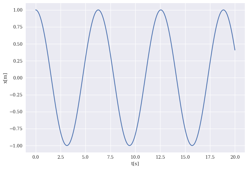
When setting up the value of \(\gamma\) we see that for \(\gamma=0\) we get the simple oscillatory motion with no damping. Choosing \(\gamma < 1\) leads to the classical underdamped case with oscillatory motion, but where the motion comes to an end.
Choosing \(\gamma =1\) leads to what normally is called critical damping and \(\gamma> 1\) leads to critical overdamping. Try it out and try also to change the initial position and velocity. Setting \(\gamma=1\) yields a situation, as discussed above, where the solution approaches quickly zero and does not oscillate. With zero initial velocity it will never cross zero.
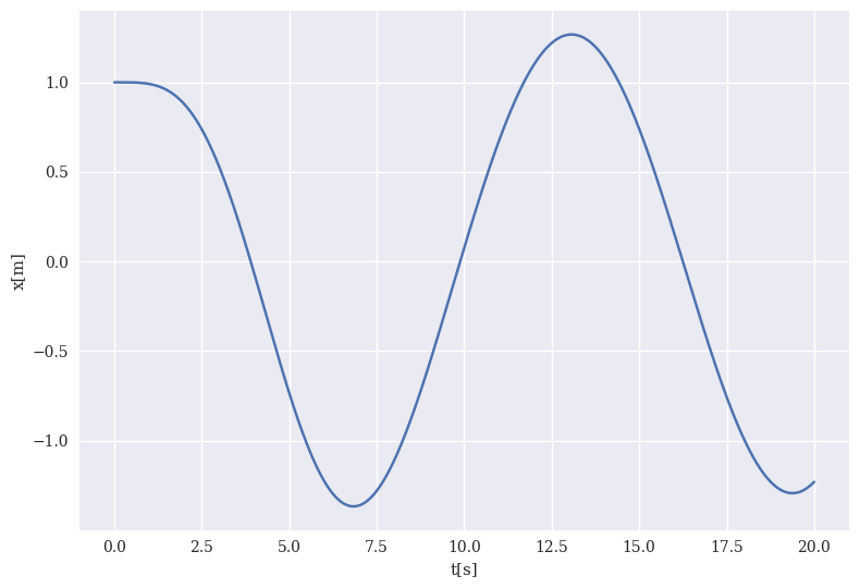
Numerical Studies of Driven Oscillations#
Solving the problem of driven oscillations numerically gives us much more flexibility to study different types of driving forces. We can reuse our earlier code by simply adding a driving force. If we stay in the \(x\)-direction only this can be easily done by adding a term \(F_{\mathrm{ext}}(x,t)\). Note that we have kept it rather general here, allowing for both a spatial and a temporal dependence.
Before we dive into the code, we need to briefly remind ourselves about the equations we started with for the case with damping, namely
with no external force applied to the system.
Let us now for simplicty assume that our external force is given by
where \(F_0\) is a constant (what is its dimension?) and \(\omega\) is the frequency of the applied external driving force. Small question: would you expect energy to be conserved now?
Introducing the external force into our lovely differential equation and dividing by \(m\) and introducing \(\omega_0^2=\sqrt{k/m}\) we have
Thereafter we introduce a dimensionless time \(\tau = t\omega_0\) and a dimensionless frequency \(\tilde{\omega}=\omega/\omega_0\). We have then
Introducing a new amplitude \(\tilde{F} =F_0/(m\omega_0^2)\) (check dimensionality again) we have
Our final step, as we did in the case of various types of damping, is to define \(\gamma = b/(2m\omega_0)\) and rewrite our equations as
This is the equation we will code below using the Euler-Cromer method.
# Common imports
import numpy as np
import pandas as pd
from math import *
import matplotlib.pyplot as plt
import os

# Where to save the figures and data files
PROJECT_ROOT_DIR = "Results"
FIGURE_ID = "Results/FigureFiles"
DATA_ID = "DataFiles/"

if not os.path.exists(PROJECT_ROOT_DIR):
    os.mkdir(PROJECT_ROOT_DIR)

if not os.path.exists(FIGURE_ID):
    os.makedirs(FIGURE_ID)

if not os.path.exists(DATA_ID):
    os.makedirs(DATA_ID)

def image_path(fig_id):
    return os.path.join(FIGURE_ID, fig_id)

def data_path(dat_id):
    return os.path.join(DATA_ID, dat_id)

def save_fig(fig_id):
    plt.savefig(image_path(fig_id) + ".png", format='png')


from pylab import plt, mpl
plt.style.use('seaborn')
mpl.rcParams['font.family'] = 'serif'


DeltaT = 0.001
#set up arrays
tfinal = 20 # in dimensionless time
n = ceil(tfinal/DeltaT)
# set up arrays for t, v, and x
t = np.zeros(n)
v = np.zeros(n)
x = np.zeros(n)
# Initial conditions as one-dimensional arrays of time
x0 =  1.0
v0 = 0.0
x[0] = x0
v[0] = v0
gamma = 0.2
Omegatilde = 0.5
Ftilde = 1.0
# Start integrating using Euler-Cromer's method
for i in range(n-1):
    # Set up the acceleration
    # Here you could have defined your own function for this
    a =  -2*gamma*v[i]-x[i]+Ftilde*cos(t[i]*Omegatilde)
    # update velocity, time and position
    v[i+1] = v[i] + DeltaT*a
    x[i+1] = x[i] + DeltaT*v[i+1]
    t[i+1] = t[i] + DeltaT
# Plot position as function of time
fig, ax = plt.subplots()
ax.set_ylabel('x[m]')
ax.set_xlabel('t[s]')
ax.plot(t, x)
fig.tight_layout()
save_fig("ForcedBlockEulerCromer")
plt.show()
/var/folders/rh/mck_zfls1nz00lkh8jq3cpv80000gn/T/ipykernel_62990/480274838.py:33: MatplotlibDeprecationWarning: The seaborn styles shipped by Matplotlib are deprecated since 3.6, as they no longer correspond to the styles shipped by seaborn. However, they will remain available as 'seaborn-v0_8-<style>'. Alternatively, directly use the seaborn API instead.
  plt.style.use('seaborn')
In the above example we have focused on the Euler-Cromer method. This method has a local truncation error which is proportional to \(\Delta t^2\) and thereby a global error which is proportional to \(\Delta t\). We can improve this by using the Runge-Kutta family of methods. The widely popular Runge-Kutta to fourth order or just RK4 has indeed a much better truncation error. The RK4 method has a global error which is proportional to \(\Delta t\).
Let us revisit this method and see how we can implement it for the above example.
Runge-Kutta (RK) methods are based on Taylor expansion formulae, but yield in general better algorithms for solutions of an ordinary differential equation. The basic philosophy is that it provides an intermediate step in the computation of \(y_{i+1}\).
To see this, consider first the following definitions
and
and
To demonstrate the philosophy behind RK methods, let us consider
the second-order RK method, RK2.
The first approximation consists in Taylor expanding \(f(t,y)\)
around the center of the integration interval \(t_i\) to \(t_{i+1}\),
that is, at \(t_i+h/2\), \(h\) being the step.
Using the midpoint formula for an integral,
defining \(y(t_i+h/2) = y_{i+1/2}\) and
\(t_i+h/2 = t_{i+1/2}\), we obtain
This means in turn that we have
However, we do not know the value of \(y_{i+1/2}\). Here comes thus the next approximation, namely, we use Euler’s method to approximate \(y_{i+1/2}\). We have then
This means that we can define the following algorithm for the second-order Runge-Kutta method, RK2.
and
with the final value
The difference between the previous one-step methods is that we now need an intermediate step in our evaluation, namely \(t_i+h/2 = t_{(i+1/2)}\) where we evaluate the derivative \(f\). This involves more operations, but the gain is a better stability in the solution.
The fourth-order Runge-Kutta, RK4, has the following algorithm
and
with the final result
Thus, the algorithm consists in first calculating \(k_1\) with \(t_i\), \(y_1\) and \(f\) as inputs. Thereafter, we increase the step size by \(h/2\) and calculate \(k_2\), then \(k_3\) and finally \(k_4\). The global error goes as \(O(h^4)\).
However, at this stage, if we keep adding different methods in our main program, the code will quickly become messy and ugly. Before we proceed thus, we will now introduce functions that enbody the various methods for solving differential equations. This means that we can separate out these methods in own functions and files (and later as classes and more generic functions) and simply call them when needed. Similarly, we could easily encapsulate various forces or other quantities of interest in terms of functions. To see this, let us bring up the code we developed above for the simple sliding block, but now only with the simple forward Euler method. We introduce two functions, one for the simple Euler method and one for the force.
Note that here the forward Euler method does not know the specific force function to be called. It receives just an input the name. We can easily change the force by adding another function.
def ForwardEuler(v,x,t,n,Force):
    for i in range(n-1):
        v[i+1] = v[i] + DeltaT*Force(v[i],x[i],t[i])
        x[i+1] = x[i] + DeltaT*v[i]
        t[i+1] = t[i] + DeltaT
def SpringForce(v,x,t):
#   note here that we have divided by mass and we return the acceleration
    return  -2*gamma*v-x+Ftilde*cos(t*Omegatilde)
It is easy to add a new method like the Euler-Cromer
def ForwardEulerCromer(v,x,t,n,Force):
    for i in range(n-1):
        a = Force(v[i],x[i],t[i])
        v[i+1] = v[i] + DeltaT*a
        x[i+1] = x[i] + DeltaT*v[i+1]
        t[i+1] = t[i] + DeltaT
and the Velocity Verlet method (be careful with time-dependence here, it is not an ideal method for non-conservative forces))
def VelocityVerlet(v,x,t,n,Force):
    for i in range(n-1):
        a = Force(v[i],x[i],t[i])
        x[i+1] = x[i] + DeltaT*v[i]+0.5*a*DeltaT*DeltaT
        anew = Force(v[i],x[i+1],t[i+1])
        v[i+1] = v[i] + 0.5*DeltaT*(a+anew)
        t[i+1] = t[i] + DeltaT
Finally, we can now add the Runge-Kutta2 method via a new function
def RK2(v,x,t,n,Force):
    for i in range(n-1):
# Setting up k1
        k1x = DeltaT*v[i]
        k1v = DeltaT*Force(v[i],x[i],t[i])
# Setting up k2
        vv = v[i]+k1v*0.5
        xx = x[i]+k1x*0.5
        k2x = DeltaT*vv
        k2v = DeltaT*Force(vv,xx,t[i]+DeltaT*0.5)
# Final result
        x[i+1] = x[i]+k2x
        v[i+1] = v[i]+k2v
	t[i+1] = t[i]+DeltaT
  Cell In[7], line 14
    t[i+1] = t[i]+DeltaT
    ^
TabError: inconsistent use of tabs and spaces in indentation
Finally, we can now add the Runge-Kutta2 method via a new function
def RK4(v,x,t,n,Force):
    for i in range(n-1):
# Setting up k1
        k1x = DeltaT*v[i]
        k1v = DeltaT*Force(v[i],x[i],t[i])
# Setting up k2
        vv = v[i]+k1v*0.5
        xx = x[i]+k1x*0.5
        k2x = DeltaT*vv
        k2v = DeltaT*Force(vv,xx,t[i]+DeltaT*0.5)
# Setting up k3
        vv = v[i]+k2v*0.5
        xx = x[i]+k2x*0.5
        k3x = DeltaT*vv
        k3v = DeltaT*Force(vv,xx,t[i]+DeltaT*0.5)
# Setting up k4
        vv = v[i]+k3v
        xx = x[i]+k3x
        k4x = DeltaT*vv
        k4v = DeltaT*Force(vv,xx,t[i]+DeltaT)
# Final result
        x[i+1] = x[i]+(k1x+2*k2x+2*k3x+k4x)/6.
        v[i+1] = v[i]+(k1v+2*k2v+2*k3v+k4v)/6.
        t[i+1] = t[i] + DeltaT
The Runge-Kutta family of methods are particularly useful when we have a time-dependent acceleration. If we have forces which depend only the spatial degrees of freedom (no velocity and/or time-dependence), then energy conserving methods like the Velocity Verlet or the Euler-Cromer method are preferred. As soon as we introduce an explicit time-dependence and/or add dissipitave forces like friction or air resistance, then methods like the family of Runge-Kutta methods are well suited for this. The code below uses the Runge-Kutta4 methods.
DeltaT = 0.001
#set up arrays
tfinal = 20 # in dimensionless time
n = ceil(tfinal/DeltaT)
# set up arrays for t, v, and x
t = np.zeros(n)
v = np.zeros(n)
x = np.zeros(n)
# Initial conditions (can change to more than one dim)
x0 =  1.0
v0 = 0.0
x[0] = x0
v[0] = v0
gamma = 0.2
Omegatilde = 0.5
Ftilde = 1.0
# Start integrating using the RK4 method
# Note that we define the force function as a SpringForce
RK4(v,x,t,n,SpringForce)

# Plot position as function of time
fig, ax = plt.subplots()
ax.set_ylabel('x[m]')
ax.set_xlabel('t[s]')
ax.plot(t, x)
fig.tight_layout()
save_fig("ForcedBlockRK4")
plt.show()
Example: The classical pendulum and scaling the equations#
Let us end our discussion of oscillations with another classical case, the pendulum.
The angular equation of motion of the pendulum is given by Newton’s equation and with no external force it reads
with an angular velocity and acceleration given by
and
We do however expect that the motion will gradually come to an end due a viscous drag torque acting on the pendulum. In the presence of the drag, the above equation becomes
where \(\nu\) is now a positive constant parameterizing the viscosity of the medium in question. In order to maintain the motion against viscosity, it is necessary to add some external driving force. We choose here a periodic driving force. The last equation becomes then
with \(A\) and \(\omega\) two constants representing the amplitude and the angular frequency respectively. The latter is called the driving frequency.
We define
the so-called natural frequency and the new dimensionless quantities
with the dimensionless driving frequency
and introducing the quantity \(Q\), called the quality factor,
and the dimensionless amplitude
We have
This equation can in turn be recast in terms of two coupled first-order differential equations as follows
and
These are the equations to be solved. The factor \(Q\) represents the number of oscillations of the undriven system that must occur before its energy is significantly reduced due to the viscous drag. The amplitude \(\hat{A}\) is measured in units of the maximum possible gravitational torque while \(\hat{\omega}\) is the angular frequency of the external torque measured in units of the pendulum’s natural frequency.
We need to define a new force, which we simply call the pendulum force. The only thing which changes from our previous spring-force problem is the non-linearity introduced by angle \(\theta\) due to the \(\sin{\theta}\) term. Here we have kept a generic variable \(x\) instead. This makes our codes very similar.
def PendulumForce(v,x,t):
#   note here that we have divided by mass and we return the acceleration
    return  -gamma*v-sin(x)+Ftilde*cos(t*Omegatilde)
DeltaT = 0.001
#set up arrays
tfinal = 20 # in years
n = ceil(tfinal/DeltaT)
# set up arrays for t, v, and x
t = np.zeros(n)
v = np.zeros(n)
theta = np.zeros(n)
# Initial conditions (can change to more than one dim)
theta0 =  1.0
v0 = 0.0
theta[0] = theta0
v[0] = v0
gamma = 0.2
Omegatilde = 0.5
Ftilde = 1.0
# Start integrating using the RK4 method
# Note that we define the force function as a PendulumForce
RK4(v,theta,t,n,PendulumForce)

# Plot position as function of time
fig, ax = plt.subplots()
ax.set_ylabel('theta[radians]')
ax.set_xlabel('t[s]')
ax.plot(t, theta)
fig.tight_layout()
save_fig("PendulumRK4")
plt.show()
Principle of Superposition and Periodic Forces (Fourier Transforms)#
If one has several driving forces, \(F(t)=\sum_n F_n(t)\), one can find the particular solution to each \(F_n\), \(x_{pn}(t)\), and the particular solution for the entire driving force is
This is known as the principal of superposition. It only applies when the homogenous equation is linear. If there were an anharmonic term such as \(x^3\) in the homogenous equation, then when one summed various solutions, \(x=(\sum_n x_n)^2\), one would get cross terms. Superposition is especially useful when \(F(t)\) can be written as a sum of sinusoidal terms, because the solutions for each sinusoidal (sine or cosine) term is analytic, as we saw above.
Driving forces are often periodic, even when they are not sinusoidal. Periodicity implies that for some time \(\tau\)
One example of a non-sinusoidal periodic force is a square wave. Many components in electric circuits are non-linear, e.g. diodes, which makes many wave forms non-sinusoidal even when the circuits are being driven by purely sinusoidal sources.
The code here shows a typical example of such a square wave generated using the functionality included in the scipy Python package. We have used a period of \(\tau=0.2\).
import numpy as np
import math
from scipy import signal
import matplotlib.pyplot as plt

# number of points
n = 500
# start and final times
t0 = 0.0
tn = 1.0
# Period
t = np.linspace(t0, tn, n, endpoint=False)
SqrSignal = np.zeros(n)
SqrSignal = 1.0+signal.square(2*np.pi*5*t)
plt.plot(t, SqrSignal)
plt.ylim(-0.5, 2.5)
plt.show()
For the sinusoidal example studied in the previous week the period is \(\tau=2\pi/\omega\). However, higher harmonics can also satisfy the periodicity requirement. In general, any force that satisfies the periodicity requirement can be expressed as a sum over harmonics,
We can write down the answer for \(x_{pn}(t)\), by substituting \(f_n/m\) or \(g_n/m\) for \(F_0/m\). By writing each factor \(2n\pi t/\tau\) as \(n\omega t\), with \(\omega\equiv 2\pi/\tau\),
The solutions for \(x(t)\) then come from replacing \(\omega\) with \(n\omega\) for each term in the particular solution,
Because the forces have been applied for a long time, any non-zero damping eliminates the homogenous parts of the solution, so one need only consider the particular solution for each \(n\).
The problem will considered solved if one can find expressions for the coefficients \(f_n\) and \(g_n\), even though the solutions are expressed as an infinite sum. The coefficients can be extracted from the function \(F(t)\) by
To check the consistency of these expressions and to verify Eq. (42), one can insert the expansion of \(F(t)\) in Eq. (41) into the expression for the coefficients in Eq. (42) and see whether
Immediately, one can throw away all the terms with \(g_m\) because they convolute an even and an odd function. The term with \(f_0/2\) disappears because \(\cos(n\omega t)\) is equally positive and negative over the interval and will integrate to zero. For all the terms \(f_m\cos(m\omega t)\) appearing in the sum, one can use angle addition formulas to see that \(\cos(m\omega t)\cos(n\omega t)=(1/2)(\cos[(m+n)\omega t]+\cos[(m-n)\omega t]\). This will integrate to zero unless \(m=n\). In that case the \(m=n\) term gives
and
The same method can be used to check for the consistency of \(g_n\).
Consider the driving force:
Find the Fourier coefficients \(f_n\) and \(g_n\) for all \(n\) using Eq. (42).
Only the odd coefficients enter by symmetry, i.e. \(f_n=0\). One can find \(g_n\) integrating by parts,
The first term is zero because \(\cos(n\omega t)\) will be equally positive and negative over the interval. Using the fact that \(\omega\tau=2\pi\),
More text will come here, chpater 5.7-5.8 of Taylor are discussed during the lectures. The code here uses the Fourier series discussed in chapter 5.7 for a square wave signal. The equations for the coefficients are are discussed in Taylor section 5.7, see Example 5.4. The code here visualizes the various approximations given by Fourier series compared with a square wave with period \(T=0.2\), witth \(0.1\) and max value \(F=2\). We see that when we increase the number of components in the Fourier series, the Fourier series approximation gets closes and closes to the square wave signal.
import numpy as np
import math
from scipy import signal
import matplotlib.pyplot as plt

# number of points
n = 500
# start and final times
t0 = 0.0
tn = 1.0
# Period
T =0.2
# Max value of square signal
Fmax= 2.0
# Width of signal
Width = 0.1
t = np.linspace(t0, tn, n, endpoint=False)
SqrSignal = np.zeros(n)
FourierSeriesSignal = np.zeros(n)
SqrSignal = 1.0+signal.square(2*np.pi*5*t+np.pi*Width/T)
a0 = Fmax*Width/T
FourierSeriesSignal = a0
Factor = 2.0*Fmax/np.pi
for i in range(1,500):
    FourierSeriesSignal += Factor/(i)*np.sin(np.pi*i*Width/T)*np.cos(i*t*2*np.pi/T)
plt.plot(t, SqrSignal)
plt.plot(t, FourierSeriesSignal)
plt.ylim(-0.5, 2.5)
plt.show()
Solving differential equations with Fouries series#
Material to be added.
Response to Transient Force#
Consider a particle at rest in the bottom of an underdamped harmonic oscillator, that then feels a sudden impulse, or change in momentum, \(I=F\Delta t\) at \(t=0\). This increases the velocity immediately by an amount \(v_0=I/m\) while not changing the position. One can then solve the trajectory by solving the equations with initial conditions \(v_0=I/m\) and \(x_0=0\). This gives
Here, \(\omega'=\sqrt{\omega_0^2-\beta^2}\). For an impulse \(I_i\) that occurs at time \(t_i\) the trajectory would be
where \(\Theta(t-t_i)\) is a step function, i.e. \(\Theta(x)\) is zero for \(x<0\) and unity for \(x>0\). If there were several impulses linear superposition tells us that we can sum over each contribution,
Now one can consider a series of impulses at times separated by \(\Delta t\), where each impulse is given by \(F_i\Delta t\). The sum above now becomes an integral,
The quantity \(e^{-\beta(t-t')}\sin[\omega'(t-t')]/m\omega'\Theta(t-t')\) is called a Green’s function, \(G(t-t')\). It describes the response at \(t\) due to a force applied at a time \(t'\), and is a function of \(t-t'\). The step function ensures that the response does not occur before the force is applied. One should remember that the form for \(G\) would change if the oscillator were either critically- or over-damped.
When performing the integral in Eq. (49) one can use angle addition formulas to factor out the part with the \(t'\) dependence in the integrand,
If the time \(t\) is beyond any time at which the force acts, \(F(t'>t)=0\), the coefficients \(I_c\) and \(I_s\) become independent of \(t\).
Consider an undamped oscillator (\(\beta\rightarrow 0\)), with characteristic frequency \(\omega_0\) and mass \(m\), that is at rest until it feels a force described by a Gaussian form,
For large times (\(t>>\tau\)), where the force has died off, find \(x(t)\).\ Solve for the coefficients \(I_c\) and \(I_s\) in Eq. (50). Because the Gaussian is an even function, \(I_s=0\), and one need only solve for \(I_c\),
The third step involved completing the square, and the final step used the fact that the integral
To see that this integral is true, consider the square of the integral, which you can change to polar coordinates,
Finally, the expression for \(x\) from Eq. (50) is