
Administrative
- Midterm will be given Thursday 10/29 in class
- Focus on classification problems (More details on Tuesday; review sheet)
- Read data, clean data, filter data, standardize data, model data, evaluate model with plots
- Open book, note, internet - no chatting with other students
- Changing groups: After the midterm we will put you in new groups for the rest of the semester.
- We will try to keep you with at least one other person from your current group.
- Please complete this MidSemester survey: www.egr.msu.edu/mid-semester-evaluation
- Homework 2 is graded; people did rather well. Well done!!!
From Pre-Class Assignment
Useful bits
- Making the data was relatively straightforward
- I was reminded about how to make a 3D plot and got it working
Challenging bits
- I was not able to make the 3D plot
- I don't quite understand what the SVM is doing when it makes dimensions
- I was unable to separate the ciruclar data
Reminder of the ML Paradigm
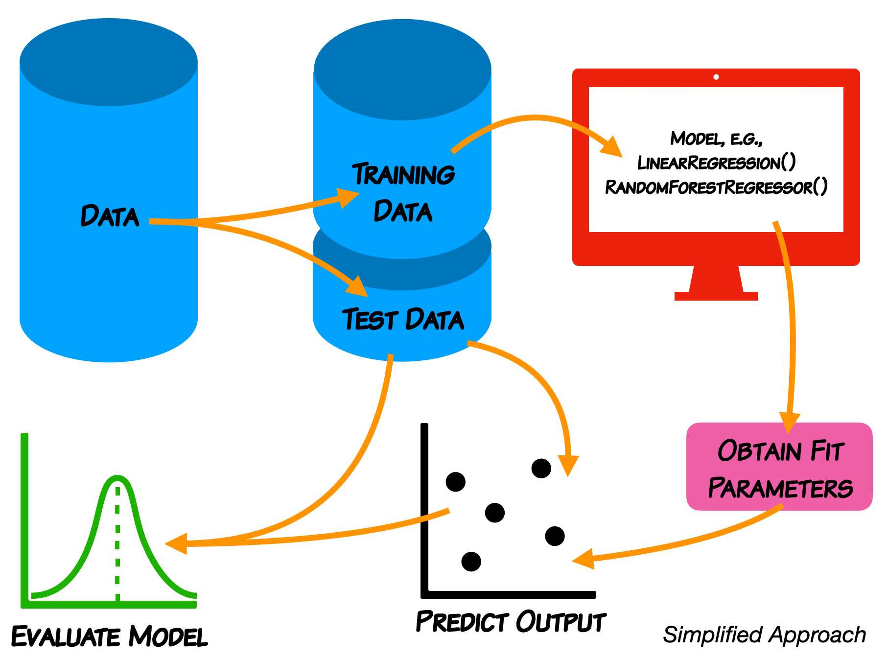
We do not expect you in this class to learn every detail of the models.
Support Vector Machines
- As a classifier, an SVM creates new dimensions from the original data, to be able to seperate the groups along the original features as well as any created dimensions.
- The kernel that we choose tells us what constructed dimensions are available to us.
We will start with a linear kernel, which tries to construct hyper-planes to seperate the data.
- For 2D, linearly separable data, this is just a line.
We are now going to use a new kernel: RBF, this will create new dimensions that aren't linear. You do not need to know the details of how this works (that is for later coursework).
We use make_circles because it gives us control over the data and it's separation; we don't have to clean or standardize it.
Let's make some circles
##imports
import numpy as np
import matplotlib.pyplot as plt
from mpl_toolkits.mplot3d import Axes3D
from sklearn.datasets import make_circles
from sklearn.svm import SVC
from sklearn.model_selection import train_test_split
from sklearn.metrics import classification_report, confusion_matrix, roc_curve, roc_auc_score

X,y = make_circles(n_samples = 100, random_state = 3)

## Plot Circles
plt.scatter(X[:,0], X[:,1], c=y)
plt.xlabel(r'$x_0$'); plt.ylabel(r'$x_1$')

Let's look at the data in 3D
fig = plt.figure(figsize = (10, 7))
ax = plt.axes(projection ="3d")

ax.scatter3D(X[:,0], X[:,1], 0, c=y)

Let's make a little more data
X,y = make_circles(n_samples = 1000, random_state = 3)

## Plot Blobs
plt.scatter(X[:,0], X[:,1], c=y)
plt.xlabel(r'$x_0$'); plt.ylabel(r'$x_1$')

Let's train up a linear SVM
- This is what we did last class; but now we have split the data
## Split the data
train_vectors, test_vectors, train_labels, test_labels = train_test_split(X, y, test_size=0.25)

## Fit with a linear kernel
cls = SVC(kernel="linear", C=10)
cls.fit(train_vectors,train_labels)

## Print the accuracy
print('Accuracy: ', cls.score(test_vectors, test_labels))
Let's check the report and confusion matrix
- We want more details than simply accuracy
## Use the model to predict
y_pred = cls.predict(test_vectors)

print("Classification Report:\n", classification_report(test_labels, y_pred))

print("Confusion Matrix:\n", confusion_matrix(test_labels, y_pred))
Let's look at the ROC curve and compute the AUC
## Construct the ROC and the AUC
fpr, tpr, thresholds = roc_curve(test_labels, y_pred)
auc = np.round(roc_auc_score(test_labels, y_pred),3)

plt.plot(fpr,tpr)
plt.plot([0,1],[0,1], 'k--')
plt.xlabel('FPR'); plt.ylabel('TPR'); plt.text(0.6,0.2, "AUC:"+str(auc));

Train the model and start evaluating it
## Fit with a RBF kernel
cls_rbf = SVC(kernel="rbf", C=10)
cls_rbf.fit(train_vectors,train_labels)

## Print the accuracy
print('Accuracy: ', cls_rbf.score(test_vectors, test_labels))
Use the model to predict and report out
## Use the model to predict
y_pred = cls_rbf.predict(test_vectors)

print("Classification Report:\n", classification_report(test_labels, y_pred))

print("Confusion Matrix:\n", confusion_matrix(test_labels, y_pred))
Construct the ROC and the AUC
## Construct the ROC and the AUC
fpr, tpr, thresholds = roc_curve(test_labels, y_pred)
auc = np.round(roc_auc_score(test_labels, y_pred),3)

plt.plot(fpr,tpr)
plt.plot([0,1],[0,1], 'k--')
plt.xlabel('FPR'); plt.ylabel('TPR'); plt.text(0.6,0.2, "AUC:"+str(auc));

Today
- We are going to use SVM with real data. We are going to use the linear kernel again, but you can change to RBF (it will take much longer to run).
- We are also going to introduce hyper-parameter optimization and grid searching (again takes more time)
In the construction of the SVM: cls = svm.SVC(kernel="linear", C=10), C is a hyperparameter that we can adjust. sklearn has a mechanism to do this automatically via a search and find the "best" choice: GridSearchCV.
Please ask lots of questions about what the code is doing today because you are not writing a lot of code today!