
Administrative
- Homework 3 will be assigned Friday 10/9 and due Friday 10/23
- Midterm will be given Thursday 10/29 in class
From Pre-Class Assignment
Useful Stuff
- Videos from Google were helpful to understand the scope of Machine Learning
- I have a better understanding of train/test split
Challenging bits
- I am still a little confused about why we split the data
- I am not sure what
make_classificationis doing - What are redundant and informative features? How do we see them in the plots?
We will be doing classification tasks for a few weeks, so we will get lots of practice
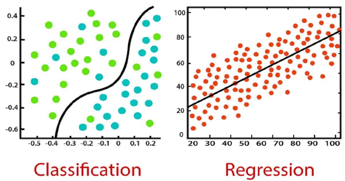
Machine Learning

Classification
Classification Algorithms
- Logistic Regression: The most traditional technique; was developed and used prior to ML; fits data to a "sigmoidal" (s-shaped) curve; fit coefficients are interpretable
- K Nearest Neighbors (KNN): A more intuitive method; nearby points are part of the same class; fits can have complex shapes
- Support Vector Machines (SVM): Developed for linear separation (i.e., find the optimal "line" to separate classes; can be extended to curved lines through different "kernels"
- Decision Trees: Uses binary (yes/no) questions about the features to fit classes; can be used with numerical and categorical input
- Random Forest: A collection of randomized decision trees; less prone to overfitting than decision trees; can rank importance of features for prediction
- Gradient Boosted Trees: An even more robust tree-based algorithm
We will learn Logisitic Regression, KNN, and SVM, but sklearn provides access to the other three methods as well.
Generate some data
make_classification lets us make fake data and control the kind of data we get.
n_features- the total number of features that can be used in the modeln_informative- the total number of features that provide unique information for classes- say 2, so $x_0$ and $x_1$
n_redundant- the total number of features that are built from informative features (i.e., have redundant information)- say 1, so $x_2 = c_0 x_0 + c_1 x_1$
n_class- the number of class labels (default 2: 0/1)n_clusters_per_class- the number of clusters per class
In [63]:
import matplotlib.pyplot as plt
plt.style.use('seaborn-colorblind')
from sklearn.datasets import make_classification

features, class_labels = make_classification(n_samples = 1000,
                                             n_features = 3,
                                             n_informative = 2,
                                             n_redundant = 1,
                                             n_clusters_per_class=1,
                                             random_state=201)
In [64]:
## Let's look at these 3D data
from mpl_toolkits.mplot3d import Axes3D
fig = plt.figure(figsize=(8,8))
ax = Axes3D(fig, rect=[0, 0, .95, 1], elev=30, azim=135)

xs = features[:, 0]
ys = features[:, 1]
zs = features[:, 2]

ax.scatter3D(xs, ys, zs, c=class_labels, ec='k')
ax.set_xlabel('feature 0')
ax.set_ylabel('feature 1')
ax.set_zlabel('feature 2')
Out[64]:

In [65]:
## From a different angle, we see the 2D nature of the data
fig = plt.figure(figsize=(8,8))
ax = Axes3D(fig, rect=[0, 0, .95, 1], elev=15, azim=90)

xs = features[:, 0]
ys = features[:, 1]
zs = features[:, 2]

ax.scatter3D(xs, ys, zs, c=class_labels, ec = 'k')
ax.set_xlabel('feature 0')
ax.set_ylabel('feature 1')
ax.set_zlabel('feature 2')
Out[65]:

Feature Subspaces
For higher dimensions, we have take 2D slices of the data (called "projections" or "subspaces")
In [66]:
f, axs = plt.subplots(1,3,figsize=(15,4))
plt.subplot(131)
plt.scatter(features[:, 0], features[:, 1], marker = 'o', c = class_labels, ec = 'k')
plt.xlabel('feature 0')
plt.ylabel('feature 1')

plt.subplot(132)
plt.scatter(features[:, 0], features[:, 2], marker = 'o', c = class_labels, ec = 'k')
plt.xlabel('feature 0')
plt.ylabel('feature 2')

plt.subplot(133)
plt.scatter(features[:, 1], features[:, 2], marker = 'o', c = class_labels, ec = 'k')
plt.xlabel('feature 1')
plt.ylabel('feature 2')

plt.tight_layout()

What about Logistic Regression?
Logistic Regression attempts to fit a sigmoid (S-shaped) function to your data. This shapes assumes that the probability of finding class 0 versus class 1 increases as the feature changes value.
In [70]:
f, axs = plt.subplots(1,3,figsize=(15,4))
plt.subplot(131)
plt.scatter(features[:,0], class_labels, c=class_labels, ec='k')
plt.xlabel('feature 0')
plt.ylabel('class label')

plt.subplot(132)
plt.scatter(features[:,1], class_labels, c=class_labels, ec='k')
plt.xlabel('feature 1')
plt.ylabel('class label')

plt.subplot(133)
plt.scatter(features[:,2], class_labels, c=class_labels, ec='k')
plt.xlabel('feature 2')
plt.ylabel('class label')

plt.tight_layout()
