Day 12 - Principal Component Analysis

Oct. 20, 2020

Administrative

• Midterm will be given Thursday 10/29 in class
  • Study Guide posted on D2L
  • Thursday: Discussion of questions for review
  • Tuesday: Midterm review assignment and discussion
• Thursday's Class:
  • We will spend the first ~1/3 of class checking in with you (re: mental health and strategies that are working)
  • We will spend the last ~2/3 brainstorming detailed questions and tasks for the review on Tuesday

Sec 003 Midterm

Classification Problem

In this midterm you will be asked to:

• Read in a data set and describe different properties of it (counts, means, etc.)
• Investigate the data for less relevant features and drop them
• Visualize feature spaces and discuss the plots
• Build a classification model using the train/test paradigm
• Evaluate and discuss the fit of model using testing data

Nearly everything we have done so far is important for your success on the midterm. But we are focused on classification and modeling with the train/test split on the midterm.

Assignments to definitely study: Day-09, Day-10, Day 11, and Day 11.5

From Pre-Class Assignment

Useful bits

• Most folks got the code working
• Videos were helpful in understanding the conceptual aspects of PCA

Challenging bits

Some really great questions:

• Why do we need to use a PCA?
• When do we use a PCA?
• What is the PCA doing with the iris data set?

Principal Component Analysis (PCA)

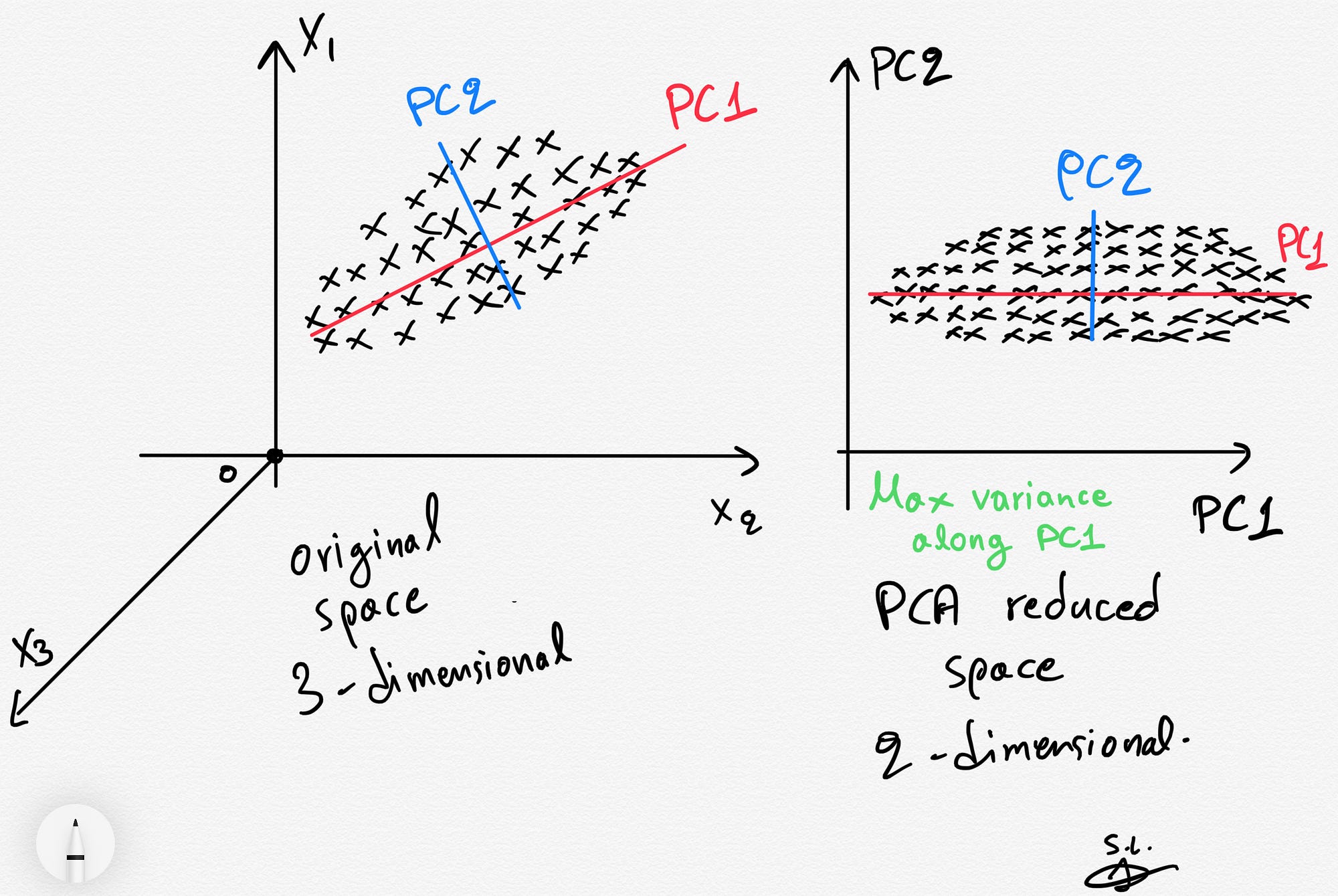
Why do we need PCA?

There are lots of reasons, but two major ones are below.

• Consider a data set with many, many features. It might be computationally intensive to perform analysis on such a large data set, so instead we use PCA to extra the major contributions to the modeled output and analyze the components instead. Benefit: less computationally intensive; quicker work
• Consider a data set with a basis that has signifcant overlap between features. That is, it's hard to tell what's important and what isn't. PCA can produce a better basis with similar (sometimes the same) information for modeling. Benefit: more meaningful features; more accurate models

Let's dive into the iris data set to see this

##imports
import numpy as np
import scipy.linalg
import sklearn.decomposition as dec
import sklearn.datasets as ds
import matplotlib.pyplot as plt
import pandas as pd

iris = ds.load_iris()
data = pd.DataFrame(iris.data, columns=['sepal_length', 'sepal_width', 'petal_length', 'petal_width'])
target = pd.DataFrame(iris.target, columns=['species'])

Let's look at the data

plt.figure(figsize=(8,5));
plt.scatter(data['sepal_length'],data['sepal_width'], c=target['species'], s=30, cmap=plt.cm.rainbow);
plt.xlabel('feature 0'); plt.ylabel('feature 1')
plt.axis([4, 8, 2, 4.5])

(4.0, 8.0, 2.0, 4.5)

Let's make a KNN classifier

from sklearn.model_selection import train_test_split
from sklearn.neighbors import KNeighborsClassifier
from sklearn.metrics import confusion_matrix, roc_curve, roc_auc_score

train_features, test_features, train_labels, test_labels = train_test_split(data,
                                                                            target['species'],
                                                                            train_size = 0.75,
                                                                            random_state=3)
neigh = KNeighborsClassifier(n_neighbors=3)
neigh.fit(train_features, train_labels)

y_predict = neigh.predict(test_features)
print(confusion_matrix(test_labels, y_predict))
print(neigh.score(test_features, test_labels))

[[15  0  0]
 [ 0 10  2]
 [ 0  0 11]]
0.9473684210526315

What happens if we use fewer features?

train_features, test_features, train_labels, test_labels = train_test_split(data.drop(columns=['petal_length','petal_width']),
                                                                            target['species'],
                                                                            train_size = 0.75,
                                                                            random_state=3)
neigh = KNeighborsClassifier(n_neighbors=3)
neigh.fit(train_features, train_labels)

y_predict = neigh.predict(test_features)
print(confusion_matrix(test_labels, y_predict))
print(neigh.score(test_features, test_labels))

[[14  1  0]
 [ 0  7  5]
 [ 0  7  4]]
0.6578947368421053

Let's do a PCA to find the principal components

pca = dec.PCA()
pca_data = pca.fit_transform(data)
print(pca.explained_variance_)

pca_data = pd.DataFrame(pca_data, columns=['PC1', 'PC2', 'PC3', 'PC4'])
plt.figure(figsize=(8,3));
plt.scatter(pca_data['PC1'], pca_data['PC2'], c=target['species'], s=30, cmap=plt.cm.rainbow);
plt.xlabel('PC1'); plt.ylabel('PC2')
plt.axis([-4, 4, -1.5, 1.5])

[4.22824171 0.24267075 0.0782095  0.02383509]

(-4.0, 4.0, -1.5, 1.5)

Let's train a KNN model

train_features, test_features, train_labels, test_labels = train_test_split(pca_data,
                                                                            target['species'],
                                                                            train_size = 0.75,
                                                                            random_state=3)
neigh = KNeighborsClassifier(n_neighbors=3)
neigh.fit(train_features, train_labels)

y_predict = neigh.predict(test_features)
print(confusion_matrix(test_labels, y_predict))
print(neigh.score(test_features, test_labels))

[[15  0  0]
 [ 0 10  2]
 [ 0  0 11]]
0.9473684210526315

Let's use only the first two principal components

train_features, test_features, train_labels, test_labels = train_test_split(pca_data.drop(columns=['PC3','PC4']),
                                                                            target['species'],
                                                                            train_size = 0.75,
                                                                            random_state=3)
neigh = KNeighborsClassifier(n_neighbors=3)
neigh.fit(train_features, train_labels)

y_predict = neigh.predict(test_features)
print(confusion_matrix(test_labels, y_predict))
print(neigh.score(test_features, test_labels))

[[15  0  0]
 [ 0 10  2]
 [ 0  0 11]]
0.9473684210526315

Questions, Comments, Concerns?